# Technical Document Extraction: State Trajectory Diagram
## 1. Image Overview
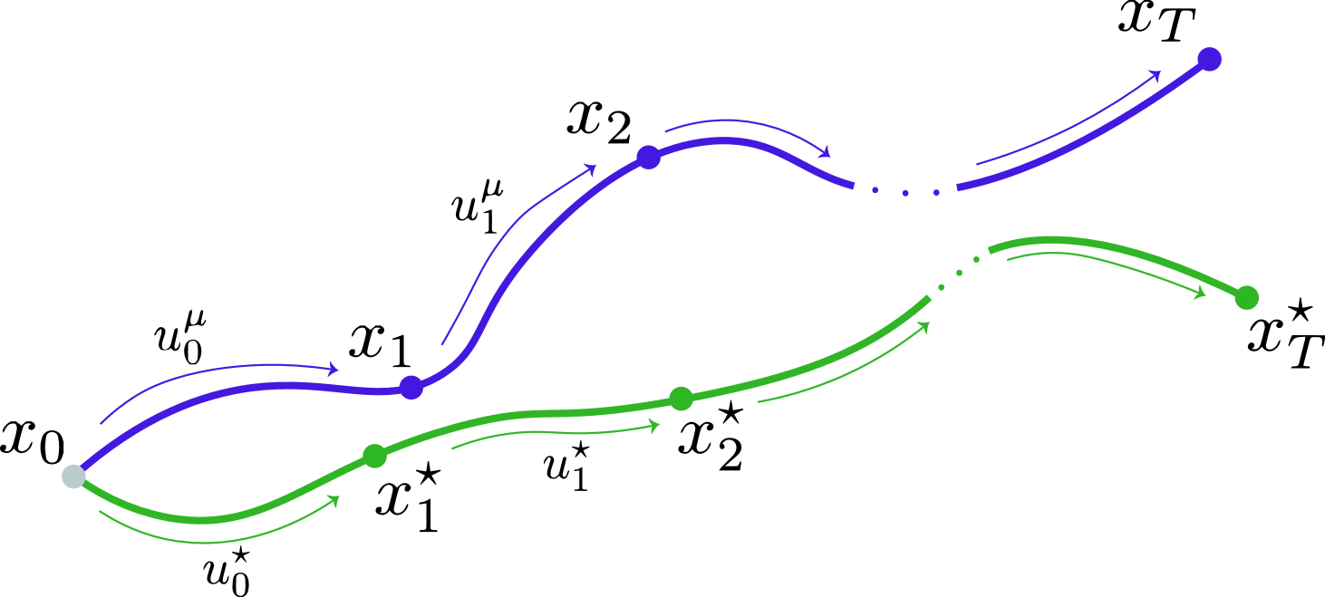
This image is a technical mathematical diagram illustrating two diverging trajectories in a state space, likely representing a control theory or reinforcement learning problem. It depicts a starting state that branches into an "optimal" or "reference" path and a "perturbed" or "actual" path over discrete time steps.
## 2. Component Isolation
### A. Starting Point (Origin)
* **Label:** $x_0$
* **Visual Marker:** A light grey solid circle.
* **Function:** This is the common initial state from which both trajectories originate.
### B. Upper Trajectory (Blue Path)
* **Color:** Solid blue line.
* **Trend:** The line slopes upward and to the right with a wavy, sinusoidal-like motion.
* **Nodes (States):**
* $x_1$: First intermediate state (blue dot).
* $x_2$: Second intermediate state (blue dot).
* $x_T$: Final state (blue dot).
* **Transitions (Control Inputs):** Represented by thin blue curved arrows above the main path.
* $u_0^\mu$: Transition from $x_0$ to $x_1$.
* $u_1^\mu$: Transition from $x_1$ to $x_2$.
* An unlabeled arrow indicates the transition from the ellipsis to $x_T$.
* **Continuity:** A break in the line is filled with three blue dots ($\dots$), indicating omitted intermediate steps between $x_2$ and $x_T$.
### C. Lower Trajectory (Green Path)
* **Color:** Solid green line.
* **Trend:** The line slopes generally rightward, staying below the blue trajectory. It exhibits a shallower curve compared to the blue path.
* **Nodes (States):**
* $x_1^\star$: First intermediate state (green dot).
* $x_2^\star$: Second intermediate state (green dot).
* $x_T^\star$: Final state (green dot).
* **Transitions (Control Inputs):** Represented by thin green curved arrows below the main path.
* $u_0^\star$: Transition from $x_0$ to $x_1^\star$.
* $u_1^\star$: Transition from $x_1^\star$ to $x_2^\star$.
* An unlabeled arrow indicates the transition from the ellipsis to $x_T^\star$.
* **Continuity:** A break in the line is filled with three green dots ($\dots$), indicating omitted intermediate steps between $x_2^\star$ and $x_T^\star$.
## 3. Mathematical Notation Summary
| Symbol | Description | Path Association |
| :--- | :--- | :--- |
| $x_0$ | Initial State | Common Origin |
| $x_t$ | State at time $t$ | Upper (Blue) |
| $x_t^\star$ | Optimal/Reference State at time $t$ | Lower (Green) |
| $u_t^\mu$ | Control input/policy $\mu$ at time $t$ | Upper (Blue) |
| $u_t^\star$ | Optimal control input at time $t$ | Lower (Green) |
| $T$ | Final time step | Both |
## 4. Logical Flow and Interpretation
The diagram visualizes the divergence between a reference trajectory (Green, denoted by $\star$) and a secondary trajectory (Blue, denoted by $\mu$).
1. Both start at $x_0$.
2. At $t=0$, applying $u_0^\star$ leads to $x_1^\star$, while applying $u_0^\mu$ leads to $x_1$.
3. This divergence continues through $t=1$ and $t=2$.
4. The trajectories conclude at different terminal states, $x_T$ and $x_T^\star$, after an undefined number of intermediate steps represented by the ellipses.