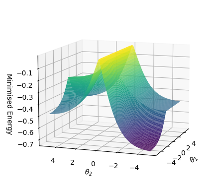
## 3D Surface Plot: Minimised Energy vs. θ₁ and θ₂ ### Overview The image displays a three-dimensional surface plot illustrating the relationship between a dependent variable, "Minimised Energy," and two independent variables, θ₁ and θ₂. The surface is rendered with a color gradient that maps directly to the energy value, providing a visual representation of the energy landscape across the parameter space defined by θ₁ and θ₂. ### Components/Axes * **Vertical Axis (Z-axis):** * **Label:** "Minimised Energy" * **Scale:** Linear, ranging from approximately **-0.7** at the bottom to **-0.1** at the top. * **Tick Marks:** Clearly marked at intervals of 0.1: -0.7, -0.6, -0.5, -0.4, -0.3, -0.2, -0.1. * **Horizontal Axis 1 (X-axis, front-left):** * **Label:** "θ₂" * **Scale:** Linear, ranging from **-4** to **4**. * **Tick Marks:** Labeled at -4, -2, 0, 2, 4. * **Horizontal Axis 2 (Y-axis, front-right):** * **Label:** "θ₁" * **Scale:** Linear, ranging from **-4** to **4**. * **Tick Marks:** Labeled at -4, -2, 0, 2, 4. * **Color Legend (Implicit):** The surface color serves as a direct legend for the "Minimised Energy" value. * **Yellow/Bright Green:** Corresponds to the highest energy values on the plot, near **-0.1**. * **Green/Teal:** Corresponds to mid-range energy values, around **-0.3 to -0.4**. * **Blue/Dark Purple:** Corresponds to the lowest energy values, near **-0.7**. ### Detailed Analysis The surface exhibits a complex, non-linear topology with distinct features: 1. **Primary Peak (Local Maximum):** A prominent, sharp peak is located near the center of the parameter space, approximately at coordinates **(θ₁ ≈ 0, θ₂ ≈ 0)**. The apex of this peak is colored bright yellow, indicating the highest "Minimised Energy" value on the plot, estimated at **≈ -0.1**. 2. **Primary Valley (Global Minimum):** A deep, broad valley is situated in the region where **θ₂ is negative** and **θ₁ is near zero**. The lowest point appears to be around **(θ₁ ≈ 0, θ₂ ≈ -4)**. This area is colored dark purple/blue, corresponding to the lowest energy value of **≈ -0.7**. 3. **Secondary Features:** * A secondary, lower ridge or shoulder extends from the main peak towards positive θ₂ values. * The surface slopes downward from the central peak in all directions, but the descent is steepest towards the primary valley (negative θ₂). * The surface appears relatively smooth, with no visible discontinuities or sharp cliffs outside of the main peak structure. **Trend Verification:** * **Series (The Surface):** The visual trend shows energy increasing to a sharp maximum at the center (θ₁=0, θ₂=0) and decreasing to a broad minimum at the edge of the plotted space (θ₁=0, θ₂=-4). The gradient is not symmetric; the drop towards negative θ₂ is more pronounced than towards positive θ₂. ### Key Observations * **Asymmetry:** The energy landscape is not symmetric about the θ₁=0 or θ₂=0 planes. The most significant feature (the deep valley) is located in the negative θ₂ half of the space. * **Single Dominant Extremum:** The plot is dominated by one clear local maximum (the peak) and one clear global minimum (the valley). * **Color-Value Correlation:** The color mapping is consistent and effectively reinforces the numerical data on the Z-axis, making the topography intuitive to read. * **Spatial Grounding:** The legend (color scale) is integrated into the surface itself. The highest point (yellow) is spatially located at the center of the θ₁-θ₂ grid. The lowest point (dark purple) is located at the front-left edge of the grid, corresponding to θ₂ = -4. ### Interpretation This plot visualizes the output of an optimization or energy minimization function over a two-dimensional parameter space (θ₁, θ₂). The "Minimised Energy" likely represents a cost function, loss function, or physical energy state that the system is trying to minimize. * **What the data suggests:** The system has a stable, low-energy configuration (the global minimum) when θ₂ is strongly negative (-4) and θ₁ is near zero. Conversely, the configuration at (θ₁=0, θ₂=0) is unstable or high-energy, representing a local maximum or a saddle point from which the system would readily "roll down" towards lower energy states. * **Relationship between elements:** The two parameters θ₁ and θ₂ are coupled in their effect on the energy. The energy is most sensitive to changes in θ₂ when θ₁ is held near zero, as evidenced by the steep gradient along the θ₂ axis at θ₁=0. * **Notable implications:** If this represents a machine learning loss landscape, training would aim to find parameters in the dark purple valley. The presence of a sharp central peak suggests a region of parameter space to avoid. The smoothness of the surface implies that gradient-based optimization methods would likely be effective. The asymmetry indicates that the parameters θ₁ and θ₂ are not interchangeable and have distinct roles in determining the system's energy.