## Scatter Plot: Principal Component Analysis of "deeper"
### Overview
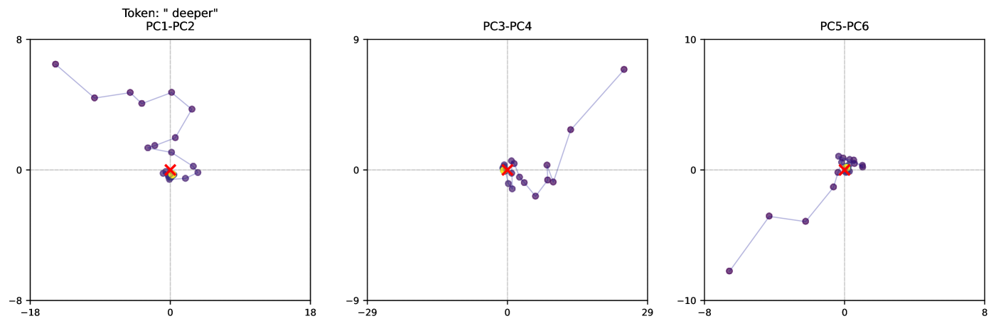
The image presents three scatter plots, each displaying the trajectory of a data point in a two-dimensional space defined by different pairs of principal components (PCs). The plots are titled "PC1-PC2", "PC3-PC4", and "PC5-PC6", and all share the title "Token: 'deeper'". Each plot shows a series of connected data points (purple dots) and a final point marked with a red 'X'. The axes are scaled differently in each plot.
### Components/Axes
* **Titles:**
* Overall Title: Token: "deeper"
* Plot 1: PC1-PC2
* Plot 2: PC3-PC4
* Plot 3: PC5-PC6
* **Axes:** Each plot has a horizontal and vertical axis.
* Plot 1 (PC1-PC2):
* X-axis (PC1): Ranges from approximately -18 to 18.
* Y-axis (PC2): Ranges from approximately -8 to 8.
* Plot 2 (PC3-PC4):
* X-axis (PC3): Ranges from approximately -29 to 29.
* Y-axis (PC4): Ranges from approximately -9 to 9.
* Plot 3 (PC5-PC6):
* X-axis (PC5): Ranges from approximately -8 to 8.
* Y-axis (PC6): Ranges from approximately -10 to 10.
* **Data Points:** Purple dots connected by light purple lines, showing the trajectory.
* **Final Point:** Marked with a red 'X' in each plot.
### Detailed Analysis
**Plot 1: PC1-PC2**
* The trajectory starts at approximately (-15, 7).
* The line moves towards the center, oscillating around (0, 0).
* The final point (red 'X') is located near the origin, approximately at (0, 0).
**Plot 2: PC3-PC4**
* The trajectory starts around (25, 8).
* The line moves towards the center, oscillating around (0, 0).
* The final point (red 'X') is located near the origin, approximately at (0, 0).
**Plot 3: PC5-PC6**
* The trajectory starts around (-7, -8).
* The line moves towards the center, oscillating around (0, 0).
* The final point (red 'X') is located near the origin, approximately at (0, 0).
### Key Observations
* All three plots show a trajectory that starts at a distance from the origin and converges towards the origin (0, 0).
* The scales of the axes vary significantly between the plots, indicating different variances in the principal components.
* The final point in each plot is consistently located near the origin.
### Interpretation
The plots visualize the movement of a data point in the space defined by different pairs of principal components. The convergence towards the origin in all three plots suggests that the later stages of the process represented by the "deeper" token are characterized by lower variance in these principal components. This could indicate a stabilization or convergence of the underlying process in the higher-dimensional space that the PCs represent. The different scales on the axes suggest that PC3 and PC4 (Plot 2) have the largest variance, while PC5 and PC6 (Plot 3) have the smallest. The red 'X' likely represents the final state of the token "deeper" after some process or transformation.