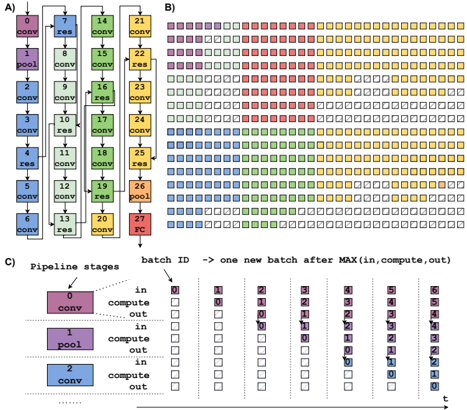
## Neural Network Pipeline Diagrams ### Overview The image presents three diagrams illustrating different aspects of a neural network pipeline. Diagram A shows the architecture of a convolutional neural network (CNN). Diagram B visualizes the processing of batches through the network. Diagram C details the pipeline stages and batch processing flow. ### Components/Axes **Diagram A: CNN Architecture** * **Nodes:** Represent layers in the CNN. Each node is labeled with a number (0-27) and a layer type (conv, pool, res, FC). * **Layer Types:** * `conv`: Convolutional layer * `pool`: Pooling layer * `res`: Residual block * `FC`: Fully connected layer * **Connections:** Arrows indicate the flow of data between layers. Some arrows bypass layers, indicating residual connections. * **Color Coding:** Each layer type is associated with a color: * `conv`: Blue, Green, Yellow * `pool`: Purple * `res`: Light Green, Light Pink * `FC`: Red **Diagram B: Batch Processing Visualization** * **Grid:** Represents the processing of batches through the network over time. * **Squares:** Each square represents a batch at a specific stage of processing. * **Color Coding:** The colors of the squares correspond to the layer types in Diagram A. * **Empty Squares:** Represent idle or unprocessed batches. **Diagram C: Pipeline Stages and Batch Flow** * **Pipeline Stages:** Shows three stages: `conv`, `pool`, and `conv`. * **Batch ID:** Indicates the ID of each batch. * **Processing Steps:** Each stage has "in," "compute," and "out" steps. * **Time (t):** Represents the progression of time from left to right. * **Arrows:** Indicate the movement of batches through the pipeline. ### Detailed Analysis **Diagram A: CNN Architecture** * The network starts with a convolutional layer (0) followed by a pooling layer (1) and then a series of convolutional and residual blocks. * Residual connections are present, allowing data to bypass certain layers. For example, the output of layer 3 is added to the output of layer 7. * The network ends with a fully connected layer (27). * The sequence of layers is approximately: conv-pool-conv-conv-res-conv-res-conv-conv-res-conv-conv-res-conv-conv-res-conv-conv-res-conv-conv-res-conv-conv-res-pool-FC **Diagram B: Batch Processing Visualization** * The diagram shows how batches are processed through the network in parallel. * The colors indicate the stage of processing for each batch. * The diagram illustrates the concept of pipelining, where multiple batches are processed simultaneously at different stages. * The first few batches are purple, then red, then yellow. * The diagram shows a total of 10 rows and approximately 25 columns. **Diagram C: Pipeline Stages and Batch Flow** * The diagram illustrates the flow of batches through a three-stage pipeline. * Each stage consists of "in," "compute," and "out" steps. * The diagram shows how batches are processed in parallel, with each stage working on a different batch at the same time. * The batches are processed in order, with batch ID increasing from left to right. * The diagram shows how a new batch is started after the maximum of the "in," "compute," and "out" times for the previous batch. ### Key Observations * **Diagram A:** The CNN architecture includes convolutional, pooling, residual, and fully connected layers. * **Diagram B:** The batch processing visualization demonstrates the pipelined execution of batches through the network. * **Diagram C:** The pipeline stages diagram illustrates the flow of batches through a three-stage pipeline. ### Interpretation The diagrams provide a comprehensive overview of a CNN pipeline, from the architecture of the network to the flow of batches through the pipeline. Diagram A shows the structure of the CNN, including the different types of layers and their connections. Diagram B visualizes the parallel processing of batches through the network, demonstrating the concept of pipelining. Diagram C provides a detailed view of the pipeline stages and the flow of batches through each stage. Together, these diagrams provide a clear understanding of how a CNN pipeline works and how it can be optimized for performance.

\n ## Diagram: Convolutional Neural Network Pipeline Visualization ### Overview The image presents a visualization of a convolutional neural network (CNN) pipeline, broken down into three parts (A, B, and C). Part A shows the network architecture with labeled layers. Part B displays a heatmap-like representation of batch processing across pipeline stages. Part C details the pipeline stages and their activity over time with a table. ### Components/Axes **Part A: Network Architecture** * Layers: "conv" (convolutional), "res" (residual), "pool" (pooling), "FC" (fully connected). * Nodes are numbered 1 through 27. * Connections indicate data flow. **Part B: Batch Processing Heatmap** * X-axis: "batch ID" – representing sequential batches processed. The arrow indicates that each batch represents the maximum of "in, compute, out". * Y-axis: Rows represent individual processing units or stages. * Colors: Represent the stage of processing (likely "in", "compute", "out"). The legend is implicit in the color scheme. * Red: Likely "in" * Yellow: Likely "compute" * Blue: Likely "out" * Green: Likely "compute" **Part C: Pipeline Stages Table** * Pipeline Stages: 0, 1, 2. * Stage 0: "conv" * Stage 1: "pool" * Stage 2: "conv" * Columns: Represent time steps (batch IDs) from 0 to 6. * Rows: Indicate the state of each pipeline stage ("in", "compute", "out") at each time step. * Colors: Correspond to the pipeline stage state. * Red: "in" * Yellow: "compute" * Blue: "out" ### Detailed Analysis or Content Details **Part A: Network Architecture** The network consists of a series of convolutional, residual, pooling, and fully connected layers. The layers are arranged in a sequential manner. * Nodes 1-3: "conv" * Node 4: "res" * Nodes 5-7: "conv" * Node 8: "pool" * Nodes 9-11: "conv" * Node 12: "res" * Nodes 13-15: "conv" * Node 16: "pool" * Nodes 17-19: "conv" * Node 20: "res" * Nodes 21-23: "conv" * Node 24: "pool" * Nodes 25-27: "conv" * Node 27: "FC" **Part B: Batch Processing Heatmap** The heatmap shows the activity of different processing units over time. * The heatmap is approximately 15 rows by 7 columns. * The first few columns (batch IDs 0-2) show predominantly red ("in") states. * As the batch ID increases, yellow ("compute") and blue ("out") states become more prevalent. * There is a staggered pattern of activity, indicating pipelining. * The heatmap shows a repeating pattern of activity across batches. **Part C: Pipeline Stages Table** The table details the state of each pipeline stage at each time step. * Stage 0 ("conv"): * Batch 0: "in" (red) * Batch 1: "compute" (yellow) * Batch 2: "out" (blue) * Batch 3-6: "in" (red) * Stage 1 ("pool"): * Batch 0: "in" (red) * Batch 1: "out" (blue) * Batch 2: "in" (red) * Batch 3: "compute" (yellow) * Batch 4: "out" (blue) * Batch 5-6: "in" (red) * Stage 2 ("conv"): * Batch 0: "in" (red) * Batch 1: "in" (red) * Batch 2: "compute" (yellow) * Batch 3: "out" (blue) * Batch 4: "in" (red) * Batch 5: "compute" (yellow) * Batch 6: "out" (blue) ### Key Observations * The pipeline operates in a staged manner, with each stage processing data sequentially. * The heatmap in Part B visually demonstrates the pipelining effect, where multiple batches are in different stages of processing simultaneously. * The table in Part C confirms the pipelining behavior, showing how each stage transitions between "in", "compute", and "out" states over time. * The network architecture in Part A provides the structural context for the pipeline visualization. ### Interpretation The image illustrates the concept of pipelining in a CNN. Pipelining allows for increased throughput by overlapping the execution of different stages of the network. The heatmap and table in Parts B and C provide a visual and tabular representation of how data flows through the pipeline, with each batch progressing through the stages concurrently. The staggered activity patterns demonstrate that while one batch is being processed in one stage, another batch may be in a different stage. This parallel processing significantly improves the efficiency of the CNN. The network architecture in Part A shows the layers that are being pipelined. The color coding consistently represents the state of each stage, making it easy to understand the flow of data. The diagram effectively communicates the benefits of pipelining in CNNs, highlighting how it enables faster and more efficient processing of data.

## Technical Diagram: Neural Network Pipeline Architecture and Batch Processing Visualization ### Overview The image is a multi-part technical diagram illustrating the architecture of a deep neural network (likely a Residual Network variant) and its corresponding batch processing pipeline over time. It consists of three labeled sections: A) Network layer architecture, B) A temporal heatmap of layer activations or computations, and C) A detailed explanation of pipeline stages and batch processing flow. ### Components/Axes **Section A: Network Architecture Diagram** * **Type:** Vertical flowchart/block diagram. * **Structure:** A sequence of 28 numbered blocks (0 to 27) arranged in a vertical column, connected by downward arrows. * **Block Labels & Types:** Each block contains a number and a text label indicating its operation type. * **Labels Found:** `conv` (convolution), `pool` (pooling), `res` (residual block), `fc` (fully connected). * **Color Coding:** Blocks are color-coded by operation type. * Purple: `conv` layers (e.g., blocks 0, 1, 3, 4, 6, 8, 10, 12, 14, 16, 18, 20, 22, 24, 27). * Blue: `pool` layers (blocks 2, 5, 13, 26). * Green: `res` (residual) blocks (blocks 7, 9, 11, 15, 17, 19, 21, 23, 25). * Orange: `fc` (fully connected) layer (block 27). * **Spatial Grounding:** The legend (color-to-operation mapping) is implicit within the diagram itself. The flow is strictly top-to-bottom. **Section B: Temporal Computation Heatmap** * **Type:** Grid/heatmap. * **Structure:** A large grid of small squares. The grid has 28 rows (corresponding to the 28 layers in Section A) and multiple columns (representing time steps or batch instances). * **Content:** Each square contains a number (matching the layer number from Section A) and is filled with a color corresponding to that layer's operation type (using the same color scheme as Section A). * **Pattern:** The grid shows a staggered, diagonal pattern of activation. For a given column (time step), not all layers are active. The pattern suggests a pipelined or wavefront execution where computation for a new batch begins before the previous batch has finished all layers. * **Spatial Grounding:** The grid is positioned to the right of Section A. The color legend is consistent with Section A. **Section C: Pipeline Stage Explanation** * **Type:** Explanatory diagram with text and schematic. * **Title:** "Pipeline stages" * **Key Text Elements:** * **Header:** `batch ID -> one new batch after MAX(in, compute, out)` * **Stage Labels:** For each layer (example shows layers 0, 1, 2), three sub-stages are listed vertically: `in`, `compute`, `out`. * **Batch ID Tracking:** A horizontal timeline (labeled `t` at the bottom right) shows the progression of batch IDs (0, 1, 2, 3, 4, 5, 6, 7) through the pipeline stages of different layers. * **Visual Flow:** Dashed lines connect the `compute` stage of one layer to the `in` stage of the next, illustrating data dependency. The diagram shows how batch 1 can start its `in` stage for layer 1 while batch 0 is still in its `compute` stage for layer 2. * **Spatial Grounding:** This section is located at the bottom of the image, below sections A and B. The explanatory text and batch ID flow are central to this section. ### Detailed Analysis **Section A - Layer Sequence:** The exact sequence of layers is: 0:conv -> 1:conv -> 2:pool -> 3:conv -> 4:conv -> 5:pool -> 6:conv -> 7:res -> 8:conv -> 9:res -> 10:conv -> 11:res -> 12:conv -> 13:pool -> 14:conv -> 15:res -> 16:conv -> 17:res -> 18:conv -> 19:res -> 20:conv -> 21:res -> 22:conv -> 23:res -> 24:conv -> 25:res -> 26:pool -> 27:fc. **Section B - Heatmap Pattern:** The heatmap visualizes the "wavefront" of computation. At an early time step (leftmost columns), only the first few layers (0, 1, 2...) are active (colored). As time progresses (moving right), the active region moves down the layers. Crucially, multiple batches are in flight simultaneously. For example, in a middle column, you might see layer 10 active for one batch while layer 5 is active for a subsequent batch. The color of each square precisely matches the color of the corresponding numbered layer in Section A. **Section C - Pipeline Mechanics:** The diagram defines three stages per layer for a batch: 1. `in`: Input data transfer/preparation. 2. `compute`: The actual computation (convolution, pooling, etc.). 3. `out`: Output data transfer/preparation. The rule `batch ID -> one new batch after MAX(in, compute, out)` indicates the system can accept a new batch once the longest of these three stages is complete for the previous batch, enabling overlap. The timeline shows batch IDs 0 through 7 progressing. Batch 1 starts its `in` stage for layer 1 at the same time batch 0 is in its `compute` stage for layer 2, demonstrating pipelining. ### Key Observations 1. **Pipelined Execution:** The core concept visualized is **pipeline parallelism**. The network layers are the pipeline stages, and multiple data batches flow through them in an overlapping fashion, increasing throughput. 2. **Color Consistency:** The color coding for operation types (`conv`=purple, `pool`=blue, `res`=green, `fc`=orange) is perfectly consistent across Sections A and B, allowing direct correlation between the architecture and its temporal execution pattern. 3. **Staggered Wavefront:** The heatmap (B) shows a clear diagonal wavefront, which is the visual signature of pipelined processing. The wavefront's slope is determined by the relative speeds of the `in`, `compute`, and `out` stages across layers. 4. **Layer Heterogeneity:** The network is not homogeneous; it mixes convolutional, pooling, and residual blocks. This heterogeneity likely leads to different `compute` times per layer, which would affect the pipeline's efficiency and the shape of the wavefront in B. 5. **Batch ID Sequencing:** Section C explicitly shows batch IDs incrementing (0,1,2,3...) and how they are staggered across the layers' stages over time (`t`). ### Interpretation This diagram is a pedagogical or technical illustration of **how to achieve high throughput in deep neural network inference or training by using pipeline parallelism**. * **What it demonstrates:** It breaks down the abstract concept into three concrete views: the static architecture (A), the dynamic execution pattern (B), and the underlying stage-level mechanics (C). It shows that by breaking the network into stages and allowing multiple batches to be processed concurrently at different stages, the hardware utilization can be increased compared to processing one batch at a time sequentially through all layers. * **Relationships:** Section A defines the *what* (the stages). Section B shows the *when* (the temporal execution). Section C explains the *how* (the rules governing stage transitions and batch acceptance). The color link between A and B is critical for understanding which part of the architecture is active at any given time. * **Notable Implications:** * The "bubble" or idle time in the pipeline would be visible in Section B as white/empty squares in the active wavefront region. The efficiency of the pipeline depends on minimizing these bubbles by balancing the `compute` times across stages. * The `MAX(in, compute, out)` rule in C is key. The pipeline's initiation interval (how often a new batch can be started) is determined by the slowest stage (`in`, `compute`, or `out`) of the bottleneck layer, not the sum of all stages. * This visualization is essential for understanding performance bottlenecks in distributed deep learning systems, where different layers might be assigned to different devices (e.g., GPUs), and communication (`in`/`out`) becomes a significant factor alongside computation.

## Diagram: Neural Network Pipeline Architecture and Processing Flow ### Overview The image depicts a technical diagram of a neural network pipeline architecture, divided into three sections (A, B, C). It combines a vertical operation sequence (A), a heatmap-style grid (B), and a temporal pipeline visualization (C). The diagram uses color-coded elements to represent computational operations, activation maps, and batch processing timelines. ### Components/Axes **Section A (Vertical Operation Sequence):** - **Vertical Axis:** Labeled with sequential numbers 0-27, representing operation stages. - **Horizontal Axis:** Unlabeled, but operations are stacked vertically. - **Legend:** - Purple = "conv" (convolution) - Green = "res" (residual connection) - Orange = "pool" (pooling) - Red = "RC" (Receptive Field?) - **Key Elements:** - Operation blocks labeled with numbers (e.g., "conv 0", "res 1", "pool 6") - Color-coded operations follow a pattern: conv → res → conv → res → pool → conv → res → RC **Section B (Heatmap Grid):** - **Grid Structure:** 28 columns (0-27) × 7 rows (0-6) - **Color Coding:** Matches Section A's legend (purple=conv, green=res, orange=pool, red=RC) - **Spatial Pattern:** - Top rows dominated by purple/green (conv/res) - Middle rows show orange/green (pool/res) - Bottom rows feature red/orange (RC/pool) - **Legend Position:** Right-aligned, matching Section A's color scheme **Section C (Temporal Pipeline):** - **Axes:** - Vertical: Time steps (t=0 to t=6) - Horizontal: Batch IDs (0-6) - **Stages:** - Purple = "conv" (input → compute → output) - Green = "pool" (input → compute → output) - Blue = "compute" (input → compute → output) - **Batch Processing:** - Each time step shows active stages for specific batches - Example: At t=0, batch 0 is in "conv" stage ### Detailed Analysis **Section A Trends:** - Operation sequence follows: conv → res → conv → res → pool → conv → res → RC - Numbers increase sequentially (0-27) with repeating patterns every 3 operations - "pool" operations occur at positions 6, 12, 18, 24 - "RC" (Receptive Field?) appears only at position 27 **Section B Heatmap Patterns:** - Color distribution suggests: - Early stages (columns 0-6) dominated by conv/res operations - Middle stages (columns 7-18) show increased pooling - Later stages (columns 19-27) feature more RC operations - Spatial correlation between Section A's operation sequence and B's column colors **Section C Pipeline Dynamics:** - Each time step processes multiple batches simultaneously - Stages overlap temporally (e.g., conv stage active for batches 0-1 at t=0) - Compute stages show delayed processing (batch 0 compute starts at t=1) - Pooling stages have longer active periods (3 time steps per batch) ### Key Observations 1. **Operation Hierarchy:** Conv → res → pool → RC forms the core processing path 2. **Temporal Parallelism:** Multiple batches process through different stages simultaneously 3. **Receptive Field Timing:** RC operation occurs only at the final time step (t=6) 4. **Batch Processing Latency:** Each batch takes 6 time steps to complete full pipeline 5. **Color Consistency:** All sections use identical color coding for operations ### Interpretation This diagram illustrates a convolutional neural network's processing pipeline with explicit temporal and spatial dimensions: 1. **Architectural Flow (A→B):** The vertical sequence in A maps directly to the heatmap columns in B, showing how operations propagate through the network 2. **Temporal Execution (C):** The pipeline visualization reveals how batches are processed through successive operations over time, with compute stages introducing latency 3. **Receptive Field Timing:** The delayed RC operation at t=6 suggests it aggregates features from all preceding operations 4. **Parallel Processing:** The grid in B demonstrates spatial activation patterns corresponding to the temporal pipeline in C The diagram emphasizes both the computational graph structure (A) and its dynamic execution characteristics (C), with B serving as a spatial activation map correlating to the temporal pipeline. The consistent color coding across all sections enables cross-referencing of operations across spatial and temporal dimensions.