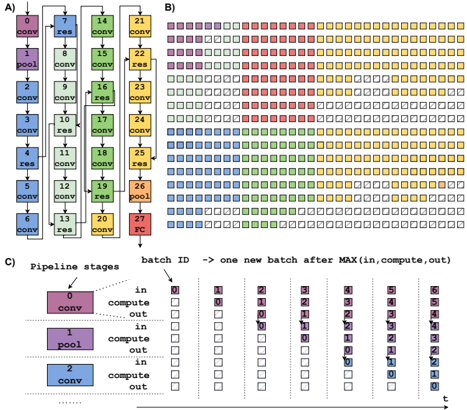
## Diagram: Neural Network Pipeline Architecture and Processing Flow ### Overview The image depicts a technical diagram of a neural network pipeline architecture, divided into three sections (A, B, C). It combines a vertical operation sequence (A), a heatmap-style grid (B), and a temporal pipeline visualization (C). The diagram uses color-coded elements to represent computational operations, activation maps, and batch processing timelines. ### Components/Axes **Section A (Vertical Operation Sequence):** - **Vertical Axis:** Labeled with sequential numbers 0-27, representing operation stages. - **Horizontal Axis:** Unlabeled, but operations are stacked vertically. - **Legend:** - Purple = "conv" (convolution) - Green = "res" (residual connection) - Orange = "pool" (pooling) - Red = "RC" (Receptive Field?) - **Key Elements:** - Operation blocks labeled with numbers (e.g., "conv 0", "res 1", "pool 6") - Color-coded operations follow a pattern: conv → res → conv → res → pool → conv → res → RC **Section B (Heatmap Grid):** - **Grid Structure:** 28 columns (0-27) × 7 rows (0-6) - **Color Coding:** Matches Section A's legend (purple=conv, green=res, orange=pool, red=RC) - **Spatial Pattern:** - Top rows dominated by purple/green (conv/res) - Middle rows show orange/green (pool/res) - Bottom rows feature red/orange (RC/pool) - **Legend Position:** Right-aligned, matching Section A's color scheme **Section C (Temporal Pipeline):** - **Axes:** - Vertical: Time steps (t=0 to t=6) - Horizontal: Batch IDs (0-6) - **Stages:** - Purple = "conv" (input → compute → output) - Green = "pool" (input → compute → output) - Blue = "compute" (input → compute → output) - **Batch Processing:** - Each time step shows active stages for specific batches - Example: At t=0, batch 0 is in "conv" stage ### Detailed Analysis **Section A Trends:** - Operation sequence follows: conv → res → conv → res → pool → conv → res → RC - Numbers increase sequentially (0-27) with repeating patterns every 3 operations - "pool" operations occur at positions 6, 12, 18, 24 - "RC" (Receptive Field?) appears only at position 27 **Section B Heatmap Patterns:** - Color distribution suggests: - Early stages (columns 0-6) dominated by conv/res operations - Middle stages (columns 7-18) show increased pooling - Later stages (columns 19-27) feature more RC operations - Spatial correlation between Section A's operation sequence and B's column colors **Section C Pipeline Dynamics:** - Each time step processes multiple batches simultaneously - Stages overlap temporally (e.g., conv stage active for batches 0-1 at t=0) - Compute stages show delayed processing (batch 0 compute starts at t=1) - Pooling stages have longer active periods (3 time steps per batch) ### Key Observations 1. **Operation Hierarchy:** Conv → res → pool → RC forms the core processing path 2. **Temporal Parallelism:** Multiple batches process through different stages simultaneously 3. **Receptive Field Timing:** RC operation occurs only at the final time step (t=6) 4. **Batch Processing Latency:** Each batch takes 6 time steps to complete full pipeline 5. **Color Consistency:** All sections use identical color coding for operations ### Interpretation This diagram illustrates a convolutional neural network's processing pipeline with explicit temporal and spatial dimensions: 1. **Architectural Flow (A→B):** The vertical sequence in A maps directly to the heatmap columns in B, showing how operations propagate through the network 2. **Temporal Execution (C):** The pipeline visualization reveals how batches are processed through successive operations over time, with compute stages introducing latency 3. **Receptive Field Timing:** The delayed RC operation at t=6 suggests it aggregates features from all preceding operations 4. **Parallel Processing:** The grid in B demonstrates spatial activation patterns corresponding to the temporal pipeline in C The diagram emphasizes both the computational graph structure (A) and its dynamic execution characteristics (C), with B serving as a spatial activation map correlating to the temporal pipeline. The consistent color coding across all sections enables cross-referencing of operations across spatial and temporal dimensions.