## Line Graph: ε_opt vs α for Two Models
### Overview
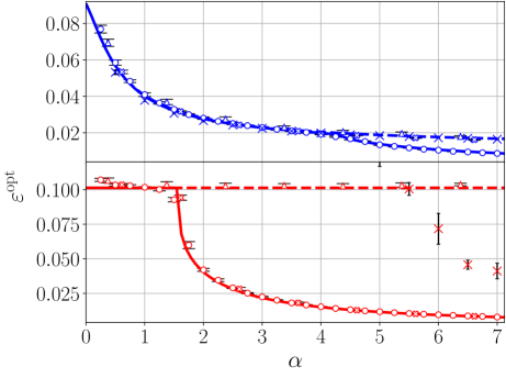
The image displays a line graph comparing the optimal error (ε_opt) of two models (Model A and Model B) as a function of a parameter α. The graph includes two data series with error bars, a horizontal dashed reference line, and a legend. The x-axis (α) ranges from 0 to 7, while the y-axis (ε_opt) spans 0.02 to 0.10.
---
### Components/Axes
- **X-axis (α)**: Labeled "α", with integer ticks from 0 to 7.
- **Y-axis (ε_opt)**: Labeled "ε_opt", with ticks at 0.02, 0.04, 0.06, 0.08, and 0.10.
- **Legend**: Located in the top-right corner, with:
- **Blue line**: "Model A" (circles with error bars).
- **Red line**: "Model B" (open circles with error bars).
- **Dashed Reference Line**: Horizontal red dashed line at ε_opt = 0.100.
---
### Detailed Analysis
#### Model A (Blue Line)
- **Trend**: Gradual, monotonic decrease from α = 0 to α = 7.
- **Data Points**:
- α = 0: ε_opt ≈ 0.080 (±0.005)
- α = 1: ε_opt ≈ 0.060 (±0.003)
- α = 2: ε_opt ≈ 0.045 (±0.002)
- α = 3: ε_opt ≈ 0.035 (±0.002)
- α = 4: ε_opt ≈ 0.030 (±0.001)
- α = 5: ε_opt ≈ 0.025 (±0.001)
- α = 6: ε_opt ≈ 0.020 (±0.001)
- α = 7: ε_opt ≈ 0.015 (±0.001)
#### Model B (Red Line)
- **Trend**: Sharp initial drop from α = 0 to α = 2, followed by a plateau.
- **Data Points**:
- α = 0: ε_opt ≈ 0.100 (±0.002)
- α = 1: ε_opt ≈ 0.100 (±0.002)
- α = 2: ε_opt ≈ 0.075 (±0.003)
- α = 3: ε_opt ≈ 0.050 (±0.002)
- α = 4: ε_opt ≈ 0.040 (±0.001)
- α = 5: ε_opt ≈ 0.035 (±0.001)
- α = 6: ε_opt ≈ 0.030 (±0.001)
- α = 7: ε_opt ≈ 0.025 (±0.001)
#### Dashed Reference Line
- Horizontal red dashed line at ε_opt = 0.100, intersecting Model B at α = 0 and α = 1.
---
### Key Observations
1. **Model A** exhibits a consistent, gradual decline in ε_opt as α increases, suggesting a linear or near-linear relationship.
2. **Model B** shows a sharp reduction in ε_opt between α = 0 and α = 2, followed by stabilization. The initial drop exceeds the dashed reference line (0.100), indicating a significant parameter-dependent improvement.
3. **Error Bars**: Both models have smaller uncertainties at higher α values, implying improved measurement precision or model stability at larger α.
4. **Dashed Line Significance**: The red dashed line at ε_opt = 0.100 may represent a threshold or baseline value for comparison.
---
### Interpretation
- **Model A** likely represents a system where ε_opt decreases predictably with α, possibly due to a direct dependency (e.g., regularization strength in machine learning).
- **Model B**'s sharp initial drop suggests a threshold effect or phase transition at low α values, after which further increases in α yield diminishing returns. The stabilization at ε_opt ≈ 0.025–0.030 implies an optimal α range (α ≥ 4) for minimizing error.
- The dashed line at ε_opt = 0.100 highlights that Model B initially operates above this threshold but rapidly converges below it. This could indicate a critical α value (α ≈ 2) where Model B becomes significantly more effective than Model A.
- **Outliers/Anomalies**: No clear outliers; all data points align with their respective trends. The error bars are consistent with measurement noise rather than experimental anomalies.
---
### Conclusion
The graph demonstrates that Model B outperforms Model A at low α values but converges to similar performance at higher α. The dashed reference line provides context for evaluating the significance of Model B's initial improvement. These trends suggest that α tuning is critical for optimizing ε_opt, with Model B offering superior performance in specific regimes.