## Line Chart: Completeness vs. Samples
### Overview
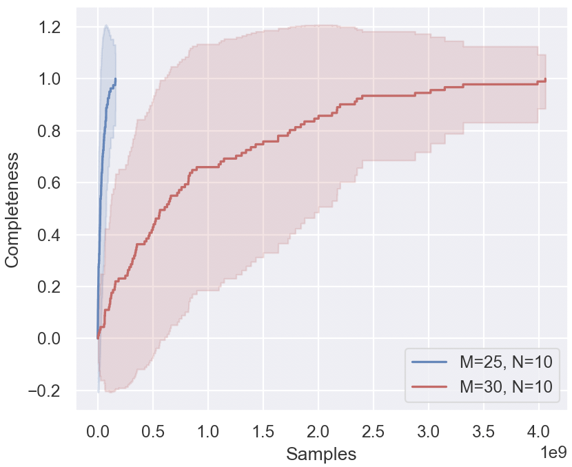
The image is a line chart comparing the completeness of two different configurations (M=25, N=10 and M=30, N=10) as a function of the number of samples. The chart displays the mean completeness for each configuration, along with a shaded region indicating the variability or uncertainty around the mean.
### Components/Axes
* **X-axis (Horizontal):** "Samples" with a scale from 0.0 to 4.0, labeled with "1e9" implying the values are in billions of samples. Axis markers are at 0.0, 0.5, 1.0, 1.5, 2.0, 2.5, 3.0, 3.5, and 4.0 (x 10^9).
* **Y-axis (Vertical):** "Completeness" with a scale from -0.2 to 1.2. Axis markers are at -0.2, 0.0, 0.2, 0.4, 0.6, 0.8, 1.0, and 1.2.
* **Legend (Bottom-Right):**
* Blue line: "M=25, N=10"
* Red line: "M=30, N=10"
* **Shaded Regions:** Each line has a corresponding shaded region around it, representing the variance or standard deviation. The blue line has a light blue shaded region, and the red line has a light red shaded region.
### Detailed Analysis
* **Blue Line (M=25, N=10):**
* Trend: The completeness increases rapidly from 0 to approximately 1.0 within the first 0.25 x 10^9 samples. After this initial rapid increase, the completeness plateaus around 1.0.
* Data Points:
* At 0 samples, completeness is approximately 0.0.
* At 0.25 x 10^9 samples, completeness is approximately 1.0.
* From 0.25 x 10^9 to 4.0 x 10^9 samples, completeness remains around 1.0.
* **Red Line (M=30, N=10):**
* Trend: The completeness increases more gradually compared to the blue line. It starts at 0 and increases steadily until it reaches approximately 0.95 around 3.0 x 10^9 samples.
* Data Points:
* At 0 samples, completeness is approximately 0.0.
* At 0.5 x 10^9 samples, completeness is approximately 0.3.
* At 1.0 x 10^9 samples, completeness is approximately 0.5.
* At 1.5 x 10^9 samples, completeness is approximately 0.65.
* At 2.0 x 10^9 samples, completeness is approximately 0.75.
* At 2.5 x 10^9 samples, completeness is approximately 0.85.
* At 3.0 x 10^9 samples, completeness is approximately 0.95.
* From 3.0 x 10^9 to 4.0 x 10^9 samples, completeness remains around 0.95.
### Key Observations
* The blue line (M=25, N=10) achieves a higher completeness value (approximately 1.0) much faster than the red line (M=30, N=10).
* The red line (M=30, N=10) increases more gradually and plateaus at a slightly lower completeness value (approximately 0.95) compared to the blue line.
* The shaded regions indicate the variability in completeness for each configuration. The blue line has a narrower shaded region, suggesting less variability compared to the red line.
### Interpretation
The chart suggests that the configuration with M=25 and N=10 (blue line) results in faster and slightly higher completeness compared to the configuration with M=30 and N=10 (red line). The narrower shaded region for the blue line indicates that the completeness achieved with M=25 and N=10 is more consistent across different runs or trials. The data demonstrates that the choice of configuration parameters (M and N) significantly impacts the completeness and stability of the system being evaluated. The initial rapid increase in completeness for M=25, N=10 suggests a faster learning or convergence rate compared to M=30, N=10.