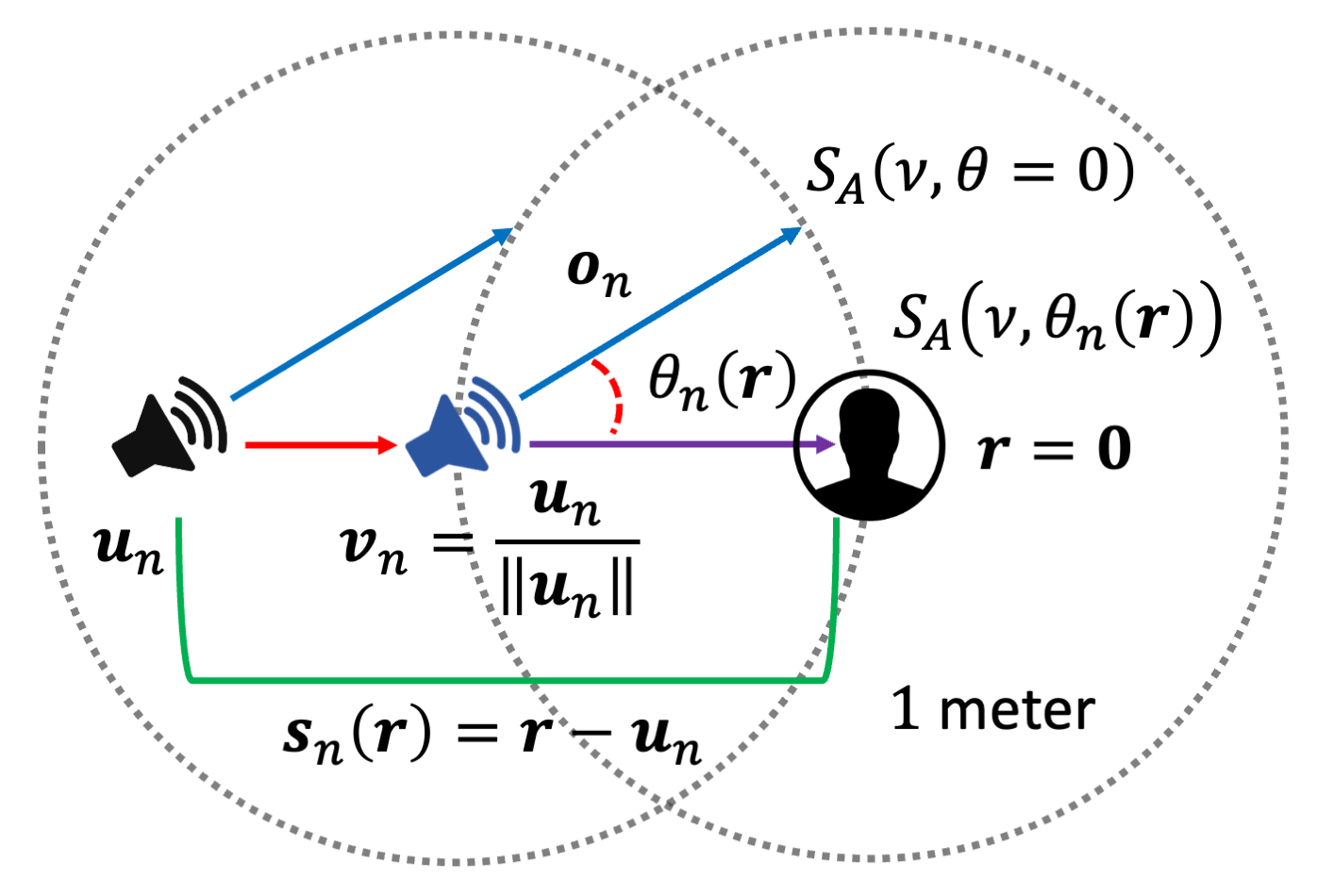
\n ## Diagram: Sound Source and Receiver Geometry ### Overview The image is a diagram illustrating the geometry of a sound source and a receiver within a spherical coordinate system. It depicts a sound source emitting waves towards a receiver (represented by a head silhouette), with annotations defining vectors, distances, and a spherical boundary. The diagram appears to be related to acoustic modeling or sound field analysis. ### Components/Axes The diagram includes the following components: * **Sound Source:** Represented by a speaker icon on the left side of the diagram. * **Receiver:** Represented by a head silhouette on the right side of the diagram. * **Spherical Boundary:** A dashed circle surrounding the sound source and receiver, labeled "1 meter". * **Vectors:** * `u_n`: A green vector pointing from the sound source towards the center of the sphere. * `o_n`: A light blue vector pointing from the sound source towards the receiver. * `v_n`: A red vector, representing the normalized `u_n` vector. * **Distance:** `r`, representing the distance from the sound source to the receiver. * **Angle:** `θ_n(r)`, representing the angle between `o_n` and `u_n`. * **Equations:** * `s_n(r) = r - u_n` * `S_A(v, θ = 0)` * `S_A(v, θ_n(r))` * **Point:** `r = 0` at the receiver location. ### Detailed Analysis / Content Details The diagram defines a coordinate system centered on the sound source. The spherical boundary has a radius of approximately 1 meter. * **Vector `u_n`:** Points radially outward from the sound source. Its length is not explicitly defined, but it appears to be a unit vector based on the normalization to `v_n`. * **Vector `v_n`:** Is defined as `u_n` normalized by its magnitude: `v_n = u_n / ||u_n||`. This implies `v_n` is a unit vector in the same direction as `u_n`. * **Vector `o_n`:** Points from the sound source to the receiver. * **Angle `θ_n(r)`:** Is the angle between the vectors `o_n` and `u_n`. It is a function of the distance `r`. * **Equation `s_n(r) = r - u_n`:** Represents a vector difference between the distance `r` and the vector `u_n`. * **Equations `S_A(v, θ = 0)` and `S_A(v, θ_n(r))`:** These equations likely represent some acoustic property (possibly sound pressure or intensity) as a function of velocity `v` and angle `θ`. The first equation is evaluated at `θ = 0`, and the second at `θ_n(r)`. * **Point `r = 0`:** Indicates that the receiver is located at the origin of the coordinate system, relative to the sound source. ### Key Observations The diagram focuses on the relationship between the sound source, receiver, and the direction of sound propagation. The use of spherical coordinates suggests an analysis of sound fields in a three-dimensional space. The equations `S_A` suggest a model for calculating some acoustic property based on the angle of incidence. ### Interpretation This diagram likely represents a simplified model for analyzing sound propagation from a source to a receiver. The equations and vectors are used to define the geometry and potentially calculate the sound pressure or intensity at the receiver. The normalization of `u_n` to `v_n` suggests a focus on the direction of sound propagation rather than its magnitude. The equations `S_A` are likely part of a larger model for predicting sound fields, potentially used in applications such as room acoustics, noise control, or audio engineering. The diagram is a conceptual representation and does not provide specific numerical data, but rather defines the relationships between the variables involved in the acoustic model. The use of `r=0` at the receiver suggests a coordinate transformation where the receiver is the origin. The diagram is a foundational element for understanding the mathematical framework used to model sound propagation.