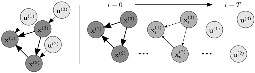
## Diagram: Dynamic System with State Variables and External Inputs ### Overview The image is a technical diagram illustrating a dynamic system composed of state variables (denoted by `x`) and external inputs (denoted by `u`). It is divided into two distinct panels by a vertical line. The left panel shows a static, instantaneous relationship graph. The right panel depicts the temporal evolution of the system's state variables from an initial time `t=0` to a final time `t=T`, while the external inputs are shown as separate, constant entities at the final time. ### Components/Axes **Left Panel (Static Graph):** * **Nodes (State Variables):** Three dark gray circles labeled `x^(1)`, `x^(2)`, and `x^(3)`. * **Nodes (External Inputs):** Three light gray circles labeled `u^(1)`, `u^(2)`, and `u^(3)`. * **Edges (Directed Relationships):** * Solid black arrows connect the state variables: `x^(1)` → `x^(3)`, `x^(3)` → `x^(2)`, `x^(2)` → `x^(1)`. * Dotted black arrows connect external inputs to state variables: `u^(1)` → `x^(1)`, `u^(2)` → `x^(2)`, `u^(3)` → `x^(3)`. **Right Panel (Temporal Evolution):** * **Temporal Axis:** An arrow at the top points from left to right, labeled `t = 0` at the start and `t = T` at the end. * **State Variable Nodes at t=0:** Three dark gray circles in a triangular formation, labeled `x^(1)`, `x^(2)`, and `x^(3)`. They are connected by solid black arrows in a cycle: `x^(1)` → `x^(3)`, `x^(3)` → `x^(2)`, `x^(2)` → `x^(1)`. * **Ellipses:** The symbol `...` appears twice, indicating intermediate time steps between `t=0`, an intermediate state, and `t=T`. * **State Variable Nodes at Intermediate Time:** Three dark gray circles labeled `x_t^(1)`, `x_t^(2)`, and `x_t^(3)`. They are connected by solid black arrows in the same cyclic pattern as at `t=0`. * **State Variable Nodes at t=T:** The state variable nodes are absent from the final panel. * **External Input Nodes at t=T:** Three light gray circles, positioned separately on the right side, labeled `u^(1)`, `u^(2)`, and `u^(3)`. They are not connected by any arrows in this panel. ### Detailed Analysis **Spatial Grounding & Component Isolation:** 1. **Header Region (Temporal Axis):** The top of the right panel contains the time progression indicator `t = 0` → `t = T`. 2. **Main Chart Region (Left Panel - Static View):** This is a complete directed graph. The state variables (`x`) form a closed loop (a cycle). Each external input (`u`) has a one-way, dotted connection to a specific state variable. 3. **Main Chart Region (Right Panel - Temporal View):** This panel is segmented into three time phases: * **Initial State (t=0, Left):** Shows the initial configuration of the state variables and their internal cyclic relationships. * **Intermediate State (Center):** Shows the state variables at some time `t`, denoted with a subscript `_t`. The internal cyclic structure is preserved. * **Final State (t=T, Right):** Only the external inputs (`u^(1)`, `u^(2)`, `u^(3)`) are displayed. The state variables are not shown, implying their values at `t=T` are the result of the process but are not explicitly diagrammed here. **Flow and Relationships:** * The diagram contrasts two views: a **structural view** (left) showing all components and their connection types, and a **temporal view** (right) showing how the state variables evolve while the external inputs are presented as constant, exogenous factors at the end of the timeline. * The solid arrows represent internal dynamics or couplings between state variables. * The dotted arrows represent external influences or control inputs acting on specific state variables. ### Key Observations * **Consistency of Internal Structure:** The cyclic relationship between `x^(1)`, `x^(2)`, and `x^(3)` is identical in the static graph and at both `t=0` and the intermediate time `t` in the temporal view. * **Separation of Concerns:** The diagram explicitly separates the system's internal state dynamics (the `x` cycle) from its external drivers (the `u` nodes). * **Temporal Abstraction:** The right panel abstracts away the specific values of the state variables at `t=T`, focusing instead on the presence of the external inputs. The ellipses (`...`) indicate a continuous or multi-step process between the shown time points. * **Labeling Convention:** State variables use superscripts `(1), (2), (3)` for identification. The temporal view adds a subscript `_t` to denote the variable's value at an intermediate time. ### Interpretation This diagram is a conceptual model for a **dynamic system with feedback and external control**. It is likely used in fields like control theory, systems biology, or network dynamics. * **What it demonstrates:** It illustrates a system where three state variables (`x`) influence each other in a closed loop (feedback cycle). Simultaneously, each state variable is independently influenced by an external input (`u`). The right panel emphasizes that this is a process unfolding over time, driven by these persistent external inputs. * **Relationship between elements:** The external inputs (`u`) are the exogenous drivers or control signals. The state variables (`x`) are the endogenous, evolving components of the system. The solid arrows define the system's internal architecture, while the dotted arrows define how it is perturbed or controlled from the outside. * **Notable implication:** The absence of the `x` nodes at `t=T` is significant. It suggests the diagram's purpose is to show the *process* of evolution (from `t=0` through intermediate `t`) under the influence of `u`, rather than to specify the final state. The final state is implied to be the outcome of applying the inputs `u` over the time interval `T` to the initial state via the defined dynamics. The diagram defines the model structure and the input scenario, not the numerical solution.