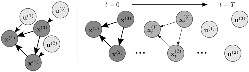
## Diagram: Dynamic System Evolution Over Time ### Overview The diagram illustrates a dynamic system evolving from an initial state at time `t = 0` to a final state at time `t = T`. It depicts nodes labeled `x(1)`, `x(2)`, `x(3)` (system states) and `u(1)`, `u(2)`, `u(3)` (external inputs or controls), connected by directional arrows indicating transitions or dependencies. The system progresses through discrete time steps, with intermediate states marked as `x_t(1)`, `x_t(2)`, `x_t(3)` at time `t`. --- ### Components/Axes - **Nodes**: - **System States**: `x(1)`, `x(2)`, `x(3)` (dark gray circles at `t = 0`; lighter gray circles at `t = T`). - **Inputs/Controls**: `u(1)`, `u(2)`, `u(3)` (light gray circles at `t = 0` and `t = T`). - **Arrows**: - Solid arrows: Represent deterministic transitions between system states (e.g., `x(1) → x(2)`). - Dashed arrows: Represent probabilistic or external influences from inputs (e.g., `u(1) → x(3)`). - **Timeline**: - Horizontal axis labeled `t = 0` (left) to `t = T` (right), indicating temporal progression. - Intermediate states at time `t` are denoted as `x_t(1)`, `x_t(2)`, `x_t(3)`. --- ### Detailed Analysis 1. **Initial State (`t = 0`)**: - System states `x(1)`, `x(2)`, `x(3)` are interconnected via solid arrows, suggesting internal dynamics. - Inputs `u(1)`, `u(2)`, `u(3)` are connected to system states via dashed arrows, indicating external perturbations. 2. **Intermediate State (`t`)**: - System states evolve to `x_t(1)`, `x_t(2)`, `x_t(3)`, maintaining the same connectivity pattern as `t = 0`. - Inputs remain active, influencing the system via dashed arrows. 3. **Final State (`t = T`)**: - System states `x(1)`, `x(2)`, `x(3)` reappear, implying cyclical or steady-state behavior. - Inputs `u(1)`, `u(2)`, `u(3)` persist, maintaining their influence. 4. **Flow Direction**: - Arrows point from left (`t = 0`) to right (`t = T`), emphasizing temporal progression. - Dashed arrows from inputs to states suggest feedback loops or external dependencies. --- ### Key Observations - **Cyclical Behavior**: The system returns to its initial state at `t = T`, suggesting periodic or recurrent dynamics. - **Input Influence**: External inputs (`u(1)`, `u(2)`, `u(3)`) consistently affect system states across all time steps. - **State Transitions**: Solid arrows between `x(1)`, `x(2)`, `x(3)` imply deterministic relationships (e.g., state `x(1)` transitions to `x(2)` and `x(3)`). --- ### Interpretation This diagram likely represents a **state-space model** or **Markov process**, where: - **System states** (`x`) evolve deterministically over time, influenced by internal rules. - **Inputs** (`u`) act as stochastic or external drivers, perturbing the system at each time step. - The cyclical return to `t = T` suggests the system may be part of a feedback loop or control system designed to stabilize or repeat behavior. The structure aligns with applications in **control theory**, **machine learning** (e.g., recurrent neural networks), or **system dynamics**, where states and inputs interact over time. The absence of numerical values implies a conceptual or schematic representation rather than a quantitative analysis.