TECHNICAL ASSET FINGERPRINT
cc7a7ed095f17494a76b16ab
Click to view fullscreen
Press ESC or click to close
FOUND IN PAPERS
EXPERT: healer-alpha-free VERSION 1
RUNTIME: free/openrouter/healer-alpha
INTEL_VERIFIED
\n
## Technical Diagram: Convolutional Neural Network Tiling and Parallelization Strategy
### Overview
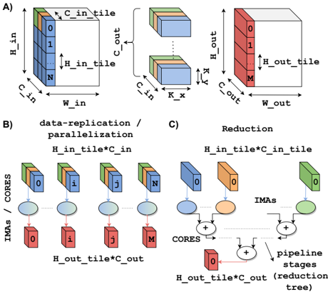
The image is a technical diagram illustrating a method for parallelizing convolutional operations in neural networks, likely for hardware acceleration. It is divided into three labeled sections (A, B, C) that depict data tiling, data replication/parallelization, and reduction stages. The diagram uses 3D block representations of data tensors and schematic flowcharts to explain the computational mapping.
### Components/Axes
The diagram contains no traditional chart axes. Its components are labeled blocks, arrows, and text annotations.
**Section A: Data Tiling**
* **Left Block (Input Tile):** A 3D rectangular prism representing an input data tile.
* **Labels:** `H_in` (height of full input), `W_in` (width of full input), `C_in` (channels of full input).
* **Sub-tile Labels:** `H_in_tile` (height of the tile), `C_in_tile` (channels of the tile). The tile is sliced along the channel dimension, with slices labeled `0`, `1`, ..., `N`.
* **Middle Block (Kernel):** A smaller 3D block representing a convolution kernel.
* **Labels:** `K_x` (kernel width), `K_y` (kernel height), `C_in` (input channels), `C_out` (output channels).
* **Right Block (Output Tile):** A 3D rectangular prism representing the resulting output data tile.
* **Labels:** `H_out` (height of full output), `W_out` (width of full output), `C_out` (channels of full output).
* **Sub-tile Label:** `H_out_tile` (height of the output tile). The tile is sliced along the output channel dimension, with slices labeled `0`, `1`, ..., `M`.
**Section B: Data-Replication / Parallelization**
* **Title:** `data-replication / parallelization`
* **Top Label:** `H_in_tile*C_in` (indicating the size of the replicated input data).
* **Components:**
* **CORES:** A row of four blue circles labeled `CORES`.
* **IMAs:** A row of four red rectangles labeled `IMAs` (likely In-Memory Arithmetic units or similar processing elements), numbered `0`, `1`, `j`, `M`.
* **Data Flow:** Each CORE is connected to an IMA. Above each CORE is a copy of the input tile from Section A (blue blocks with channel slices `0`, `i`, `j`, `N`). This shows the input tile `H_in_tile*C_in` is replicated across all cores.
* **Bottom Label:** `H_out_tile*C_out` (indicating the size of the partial output data generated per IMA).
**Section C: Reduction**
* **Title:** `Reduction`
* **Top Label:** `H_in_tile*C_in` (same as in B).
* **Components:**
* **IMAs:** Three colored rectangles (blue, orange, green) labeled `IMAs`, each with a channel slice `0`.
* **CORES:** Two blue circles labeled `CORES` below the IMAs.
* **Pipeline Stages:** A series of addition symbols (`+`) connected by arrows, forming a tree structure.
* **Bottom Label:** `H_out_tile*C_out` (the final reduced output size).
* **Annotation:** `pipeline stages (reduction tree)` points to the addition tree.
* **Flow:** Data from the IMAs flows into the CORES, then into a multi-stage addition tree (reduction tree) that sums partial results to produce the final output tile.
### Detailed Analysis
1. **Spatial Grounding & Component Isolation:**
* **Section A (Top):** Occupies the top half of the image. It defines the fundamental data structures: an input tile, a kernel, and an output tile. The spatial relationship shows the kernel operating on the input tile to produce the output tile.
* **Section B (Bottom Left):** Shows the parallelization strategy. The input tile (`H_in_tile*C_in`) is **replicated** identically to multiple processing units (CORES/IMAs). Each unit computes a different part of the output channel dimension (`0` to `M`), generating partial results of size `H_out_tile*C_out`.
* **Section C (Bottom Right):** Shows the reduction strategy. Partial results from different IMAs (represented by different colors: blue, orange, green) are **summed together** through a pipeline of adders (a reduction tree) to produce the final consolidated output tile of size `H_out_tile*C_out`.
2. **Trend Verification (Data Flow):**
* The visual trend is a **divergence then convergence** pattern.
* **Divergence (B):** A single input tile is copied (replicated) to many parallel processors.
* **Convergence (C):** The partial outputs from those many processors are combined (reduced) via summation into a single output tile.
### Key Observations
* The diagram explicitly separates the **parallelizable** part of the computation (data replication and independent partial output generation in B) from the **sequential dependency** (the reduction/summation step in C).
* The use of different colors (blue, orange, green) for IMAs in Section C is critical. It visually distinguishes partial results originating from different parallel units before they are summed. This cross-references with the multiple identical blue blocks in Section B, implying that after parallel computation, the results are distinct (hence different colors) and need reduction.
* The labels `H_in_tile*C_in` and `H_out_tile*C_out` are used consistently across B and C to denote data volume at different stages, providing a clear quantitative link between the parallelization and reduction phases.
### Interpretation
This diagram explains a **tiled, data-parallel convolution algorithm** optimized for a many-core or distributed hardware architecture (like a systolic array or in-memory computing fabric).
* **What it demonstrates:** It shows how to break a large convolution into smaller, independent tile-based computations that can be executed in parallel (Section B), and then how to correctly combine the results (Section C). This is a fundamental technique for achieving high throughput in neural network accelerators.
* **Relationship between elements:** Section A defines the problem geometry. Section B maps that geometry onto parallel hardware by replicating inputs. Section C solves the data dependency created by the parallelization, ensuring the final output is mathematically correct by summing partial results.
* **Notable pattern:** The "replicate input, reduce output" pattern is a classic strategy for parallelizing operations with a reduction dimension (like the output channel summation in convolution). The diagram highlights the hardware cost of this strategy: the need for a high-bandwidth network to replicate data (B) and a reduction network to combine results (C).
* **Underlying message:** The efficiency of this approach hinges on balancing the tile size (`H_in_tile`, `C_in_tile`) to maximize parallelism in stage B while minimizing the overhead of the reduction tree in stage C. The diagram serves as a blueprint for mapping a convolutional layer onto a specific parallel hardware substrate.
DECODING INTELLIGENCE...