## Diagram: Parallel Processing Pipeline with Data Replication and Reduction
### Overview
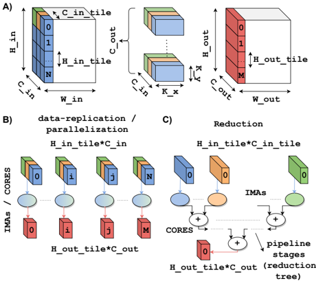
The image depicts a technical diagram of a parallel processing pipeline divided into three sections (A, B, C). It illustrates data flow through a 3D grid structure, data replication/parallelization stages, and a reduction process. The diagram uses color-coded blocks and arrows to represent data transformations and computational stages.
### Components/Axes
**Section A (3D Grid Structure):**
- **Input Tile**:
- Dimensions: `H_in_tile` (height), `W_in_tile` (width), `N` (depth)
- Labels: `C_in_tile` (channel input), `H_in_tile` (height input)
- **Output Tile**:
- Dimensions: `H_out_tile` (height), `W_out_tile` (width), `M` (depth)
- Labels: `C_out_tile` (channel output), `H_out_tile` (height output)
- **Arrows**:
- Input → Output (transformation flow)
- Color-coded: Blue (input), Green (output)
**Section B (Data-Replication/Parallelization):**
- **Blocks**:
- Labeled `0` to `N` (parallel processing units)
- Each block contains:
- `H_in_tile*C_in` (input data)
- `H_out_tile*C_out` (output data)
- **IMA Blocks**:
- Connected in a pipeline (left to right)
- Color-coded: Blue (input), Green (output), Red (intermediate)
**Section C (Reduction):**
- **IMA Blocks**:
- Connected in a tree structure (top-down)
- Color-coded: Orange (input), Green (output), Red (intermediate), Blue (final)
- **Labels**:
- "IMAs" (Intermediate Processing Units)
- "Pipeline stages (reduction tree)"
**Legend**:
- **Colors**:
- Blue: Input data (`H_in_tile*C_in`)
- Green: Output data (`H_out_tile*C_out`)
- Red: Intermediate processing
- Orange: Reduction input
- Yellow: Reduction output
### Detailed Analysis
**Section A**:
- The 3D grid structure shows a transformation from input tiles (`H_in_tile`, `W_in_tile`, `N`) to output tiles (`H_out_tile`, `W_out_tile`, `M`).
- The `C_in_tile` and `C_out_tile` labels indicate channel dimensions, suggesting a convolutional or tensor-based operation.
**Section B**:
- Parallel processing units (`0` to `N`) replicate input data (`H_in_tile*C_in`) and produce output data (`H_out_tile*C_out`).
- The IMA blocks form a linear pipeline, with each stage passing data to the next.
**Section C**:
- The reduction process uses a tree structure to combine outputs from multiple IMA blocks.
- The final output (`H_out_tile*C_out`) is aggregated through hierarchical reduction stages.
### Key Observations
1. **Data Flow**:
- Input data is first processed in parallel (Section B), then reduced hierarchically (Section C).
2. **Dimensional Changes**:
- Input and output tiles have different spatial dimensions (`W_in_tile` vs. `W_out_tile`), indicating downsampling or upsampling.
3. **Color Consistency**:
- Legend colors match component labels (e.g., blue for input, green for output).
4. **Reduction Tree**:
- The tree structure in Section C suggests logarithmic complexity for combining results.
### Interpretation
This diagram represents a **parallel computing architecture** for tensor operations, likely in machine learning or signal processing. Key insights:
- **Parallelization**: Section B enables concurrent processing of data chunks, improving throughput.
- **Reduction Efficiency**: Section C’s tree structure minimizes communication overhead by aggregating results hierarchically.
- **Dimensional Adaptation**: The change in width (`W_in_tile` → `W_out_tile`) implies spatial transformation (e.g., pooling, striding).
- **Intermediate Stages**: Red and orange blocks represent computational steps (e.g., matrix multiplications, activation functions).
The diagram emphasizes **scalability** (via parallelization) and **efficiency** (via reduction), critical for high-dimensional data processing. The use of color-coding and explicit dimensional labels ensures clarity in tracking data flow and transformations.