## Bar Charts: Relative Memory Usage and Training Time Comparison
### Overview
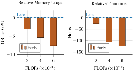
The image contains two side-by-side vertical bar charts comparing the performance of two methods, labeled "Early" and "Late," across three different computational scales measured in FLOPs (×10²¹). The charts quantify the relative difference in memory usage per GPU and training time between these methods.
### Components/Axes
**Common Elements:**
* **X-Axis (Both Charts):** Labeled "FLOPs (×10²¹)". It has three categorical tick marks at positions 2, 4, and 6, representing computational scales of 2×10²¹, 4×10²¹, and 6×10²¹ FLOPs.
* **Legend (Both Charts):** Located in the bottom-left corner of each chart's plot area. It defines two series:
* **Early:** Represented by solid brown bars.
* **Late:** Represented by a dashed blue line.
* **Baseline:** A dashed blue line labeled "Late" runs horizontally at the 0 value on the Y-axis in both charts, serving as the reference point for comparison.
**Left Chart: "Relative Memory Usage"**
* **Title:** "Relative Memory Usage" (centered at the top).
* **Y-Axis:** Labeled "GB per GPU". The scale runs from 0 at the top to -10 at the bottom, with major gridlines at 0, -5, and -10. Negative values indicate higher memory usage relative to the "Late" baseline.
**Right Chart: "Relative Train time"**
* **Title:** "Relative Train time" (centered at the top).
* **Y-Axis:** Labeled "Hours". The scale runs from 0 at the top to -150 at the bottom, with major gridlines at 0, -50, -100, and -150. Negative values indicate longer training times relative to the "Late" baseline.
### Detailed Analysis
**Left Chart: Relative Memory Usage**
* **Trend Verification:** The "Early" series (brown bars) shows a clear downward trend. As the FLOPs scale increases from 2 to 6 (×10²¹), the bars become progressively longer in the negative direction, indicating a growing memory usage penalty.
* **Data Points (Approximate):**
* At **2×10²¹ FLOPs:** The "Early" bar extends to approximately **-3.5 GB per GPU**.
* At **4×10²¹ FLOPs:** The "Early" bar extends to approximately **-5.5 GB per GPU**.
* At **6×10²¹ FLOPs:** The "Early" bar extends to approximately **-7.5 GB per GPU**.
* **"Late" Series:** The dashed blue line remains constant at **0 GB per GPU** across all FLOP scales, indicating no relative change from the baseline.
**Right Chart: Relative Train time**
* **Trend Verification:** The "Early" series (brown bars) also shows a strong downward trend. The training time penalty increases significantly with computational scale.
* **Data Points (Approximate):**
* At **2×10²¹ FLOPs:** The "Early" bar extends to approximately **-25 Hours**.
* At **4×10²¹ FLOPs:** The "Early" bar extends to approximately **-100 Hours**.
* At **6×10²¹ FLOPs:** The "Early" bar extends to approximately **-120 Hours**.
* **"Late" Series:** The dashed blue line remains constant at **0 Hours** across all FLOP scales.
### Key Observations
1. **Consistent Underperformance of "Early":** The "Early" method consistently uses more memory and takes longer to train than the "Late" method at all measured scales.
2. **Scaling Penalty:** The performance gap between "Early" and "Late" widens as the computational scale (FLOPs) increases. The penalty is not linear; the jump in training time from 2 to 4 FLOPs is particularly large.
3. **"Late" as an Optimized Baseline:** The "Late" method is presented as the optimized reference point (0 on both charts), against which the "Early" method's inefficiencies are measured.
4. **Correlated Metrics:** The trends in memory usage and training time are strongly correlated, suggesting that the factors causing increased memory consumption in the "Early" method also lead to slower training.
### Interpretation
This data demonstrates the significant efficiency gains achieved by a method or system state labeled "Late" compared to an "Early" one. The "Late" approach appears to be a highly optimized version that eliminates substantial overhead in both memory footprint and computation time.
The **Peircean investigative reading** suggests the charts are making a causal argument: adopting the "Late" methodology (the *interpretant*) resolves the inefficiencies inherent in the "Early" stage (the *object*), as evidenced by the quantitative data (the *sign*). The widening gap at higher FLOPs indicates that the optimizations in "Late" are particularly crucial for large-scale, computationally intensive tasks, where the costs of the "Early" approach become prohibitively high. The charts effectively argue for the scalability and necessity of the "Late" optimization.