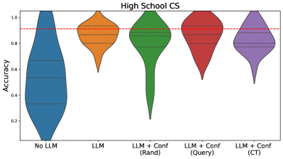
\n ## Violin Plot: High School CS Accuracy by Model Configuration ### Overview The image is a violin plot comparing the distribution of accuracy scores for five different model configurations on a "High School CS" (Computer Science) task. The plot visualizes the probability density of the data at different values, showing both the median and the spread of results for each configuration. ### Components/Axes * **Chart Title:** "High School CS" (centered at the top). * **Y-Axis:** Labeled "Accuracy". The scale runs from 0.0 to 1.0, with major tick marks at 0.0, 0.2, 0.4, 0.6, 0.8, and 1.0. * **X-Axis:** Contains five categorical labels, each corresponding to a model configuration. From left to right: 1. `No LLM` 2. `LLM` 3. `LLM + Conf (Rand)` 4. `LLM + Conf (Query)` 5. `LLM + Conf (CT)` * **Legend/Color Mapping:** The color of each violin corresponds directly to its x-axis label. There is no separate legend box; the labels are positioned directly beneath their respective plots. * `No LLM`: Blue * `LLM`: Orange * `LLM + Conf (Rand)`: Green * `LLM + Conf (Query)`: Red * `LLM + Conf (CT)`: Purple * **Reference Line:** A horizontal red dashed line is drawn across the plot at the `Accuracy = 0.9` mark. ### Detailed Analysis The analysis proceeds from left to right, isolating each component. 1. **`No LLM` (Blue, far left):** * **Trend/Shape:** The distribution is very broad and skewed towards lower accuracy. It has a wide base near 0.0 and tapers to a point near 1.0, indicating a high variance with many low scores. * **Key Values:** The median (indicated by the central horizontal line within the violin) is approximately **0.5**. The bulk of the data (the widest part of the violin) is concentrated between ~0.2 and ~0.6. 2. **`LLM` (Orange, second from left):** * **Trend/Shape:** The distribution is more concentrated and shifted upward compared to `No LLM`. It is widest in the upper half, indicating a cluster of higher scores. * **Key Values:** The median is approximately **0.8**. The distribution spans roughly from 0.6 to 0.95, with the highest density around 0.8-0.9. 3. **`LLM + Conf (Rand)` (Green, center):** * **Trend/Shape:** This distribution has a distinctive shape: a very narrow, long tail extending down to ~0.1, and a wide, dense bulb in the upper region. This suggests most runs perform very well, but a few have catastrophically low accuracy. * **Key Values:** The median is approximately **0.85**. The main cluster of data is between ~0.75 and ~0.95. The long downward tail is a notable outlier pattern. 4. **`LLM + Conf (Query)` (Red, second from right):** * **Trend/Shape:** Similar in overall shape to the green (`Rand`) plot but appears slightly more compact in its upper region and has a less extreme downward tail. * **Key Values:** The median is approximately **0.87**. The dense region is between ~0.8 and ~0.95. The lower tail extends to about 0.5. 5. **`LLM + Conf (CT)` (Purple, far right):** * **Trend/Shape:** This distribution is the most compact and highest-shifted of all. It is widest near the top, indicating high consistency in top-tier performance. * **Key Values:** The median is the highest, approximately **0.88**. The data is tightly clustered between ~0.8 and ~0.95, with a very short lower tail ending around 0.7. ### Key Observations * **Clear Performance Hierarchy:** There is a visible, step-wise improvement in median accuracy from left to right: `No LLM` < `LLM` < `LLM + Conf (Rand)` < `LLM + Conf (Query)` ≈ `LLM + Conf (CT)`. * **Variance Reduction:** As models become more sophisticated (moving right), the distributions generally become narrower (except for the specific outlier tail in `Rand`), indicating more consistent and reliable performance. * **The 0.9 Benchmark:** The red dashed line at 0.9 serves as a high-performance threshold. Only the medians of the three rightmost configurations (`Rand`, `Query`, `CT`) approach this line, with their upper distributions clearly exceeding it. * **Outlier Pattern:** The `LLM + Conf (Rand)` configuration shows a unique failure mode, with a long tail of very low accuracy scores not seen in the `Query` or `CT` variants. ### Interpretation This chart demonstrates the significant impact of using a Large Language Model (LLM) and, more importantly, applying confidence calibration techniques for a High School Computer Science task. * **Baseline vs. LLM:** The `No LLM` model performs poorly and unreliably. Simply adding an `LLM` provides a massive boost in both average accuracy and consistency. * **Value of Confidence Calibration:** All three `+ Conf` methods outperform the base `LLM`, suggesting that calibrating the model's confidence in its answers is crucial for maximizing accuracy on this task. * **Method Comparison:** While all calibration methods help, `Query` and `CT` appear superior to `Rand`. They achieve similar high median accuracy but with more stable distributions (lacking the extreme low-end failures of `Rand`). This implies that the strategy for gathering confidence information (random vs. query-based vs. the "CT" method) meaningfully affects robustness. * **Practical Implication:** For reliable deployment on this type of problem, using an LLM with a sophisticated confidence calibration method like `Query` or `CT` is recommended. The `Rand` method, while effective on average, carries a higher risk of occasional severe failure. The data suggests that near-human-level accuracy (approaching 0.9) is achievable with the right model configuration.