## Training Loss vs. FLOPS Scaling Curves
### Overview
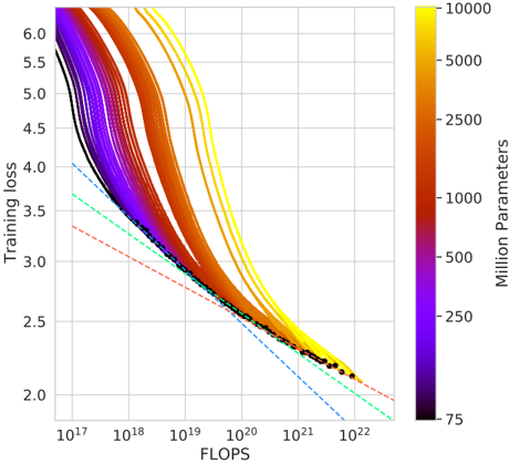
This image is a line chart illustrating the relationship between computational resources (measured in FLOPS) and model training loss for neural networks of varying sizes. The chart demonstrates scaling laws, showing how increasing compute and model parameters leads to lower loss. The data is presented as a series of colored curves, each representing a model with a specific number of parameters, plotted on a log-log scale.
### Components/Axes
* **X-Axis (Horizontal):** Labeled **"FLOPS"**. It uses a logarithmic scale with major tick marks at `10^17`, `10^18`, `10^19`, `10^20`, `10^21`, and `10^22`.
* **Y-Axis (Vertical):** Labeled **"Training loss"**. It uses a linear scale with major tick marks from `2.0` to `6.0` in increments of `0.5`.
* **Color Bar (Legend):** Located on the right side of the chart. It is labeled **"Million Parameters"** and uses a continuous color gradient to represent model size.
* **Color Scale:** Ranges from dark purple/black at the bottom to bright yellow at the top.
* **Labeled Values (from bottom to top):** `75`, `250`, `500`, `1000`, `2500`, `5000`, `10000`.
* **Data Series:** Multiple solid lines (curves) are plotted, each colored according to the color bar. Their placement corresponds to different model sizes.
* **Reference Lines:** Three dashed lines are present in the lower-left quadrant:
* A **red dashed line** with the shallowest slope.
* A **green dashed line** with a medium slope.
* A **blue dashed line** with the steepest slope.
* **Data Points:** A series of small **black dots** are plotted along the lower envelope of the curves, primarily between `10^20` and `10^22` FLOPS and between loss values of approximately `2.2` and `2.5`.
### Detailed Analysis
* **Trend Verification:** All colored curves slope downward from left to right, indicating that **Training loss decreases as FLOPS increase**. The curves are not straight lines on this log-linear plot; they are convex, showing diminishing returns.
* **Curve Behavior by Model Size (Color):**
* **Small Models (Purple/Black, ~75-500M params):** Start at a lower loss (~5.5-6.0 at 10^17 FLOPS) but have a shallower slope. They are the first to plateau.
* **Medium Models (Red/Orange, ~1000-2500M params):** Start at a moderate loss and show a steady decline.
* **Large Models (Yellow, ~5000-10000M params):** Start at the highest loss (above 6.0 at 10^17 FLOPS) but exhibit the steepest initial decline. They continue to improve at higher FLOPS where smaller models have flattened.
* **Convergence:** At very high compute (`>10^21` FLOPS), the curves for different model sizes begin to converge towards a similar loss value (approximately `2.2` to `2.4`).
* **Black Dots:** These points closely follow the lower boundary formed by the most efficient models (the yellow/orange curves) at high FLOPS, suggesting they may represent optimal or empirical data points from actual training runs.
* **Dashed Reference Lines:** These lines, originating from the left axis, represent theoretical power-law scaling relationships (Loss ∝ FLOPS^(-α)). The blue line has the steepest exponent (α), the green is intermediate, and the red has the shallowest exponent. The actual model curves are steeper than the red and green lines but less steep than the blue line at high FLOPS.
### Key Observations
1. **The "Compute-Optimal" Frontier:** The black dots and the lower envelope of the colored curves trace a frontier. To achieve a given loss with minimal FLOPS, one should follow this frontier, which involves scaling both model size and compute together.
2. **Larger Models Are More Compute-Efficient at Scale:** While large models (yellow) start with worse loss, they become more efficient at converting additional FLOPS into lower loss beyond approximately `10^19` FLOPS. Their curves are below the curves of smaller models in the high-FLOPS region.
3. **Diminishing Returns:** All curves show diminishing returns; the improvement in loss per tenfold increase in FLOPS becomes smaller as compute grows.
4. **Parameter Count vs. Performance Trade-off:** There is a clear visual trade-off: using a smaller model (purple) yields better loss at low compute (`<10^18` FLOPS), but using a larger model (yellow) is necessary to achieve the lowest possible loss at high compute (`>10^20` FLOPS).
### Interpretation
This chart is a classic visualization of **neural scaling laws**, which are empirical relationships between a model's performance (here, training loss), its size (parameters), and the amount of compute (FLOPS) used to train it.
* **What the data suggests:** The data demonstrates that performance improves predictably with both model scale and compute, following a power-law trend. The convergence of curves suggests a fundamental limit to how much loss can be reduced with more compute for a given architecture and data distribution.
* **How elements relate:** The color gradient directly links model size to the trajectory of its learning curve. The dashed lines provide a baseline for comparing the efficiency of the actual models against simple theoretical scaling. The black dots likely represent the most efficient training points discovered, forming the "Pareto frontier" of the scaling landscape.
* **Notable implications:** The key insight is that to push the state-of-the-art (to the lowest loss), one must **scale both model parameters and training compute in tandem**. Simply making a model larger without proportionally more compute, or throwing more compute at a fixed small model, is inefficient. This principle guides resource allocation in large-scale AI research. The chart argues for the development of ever-larger models, provided they are trained with commensurately vast computational resources.