## Diagram: Synaptic Input and Energy Landscape
### Overview
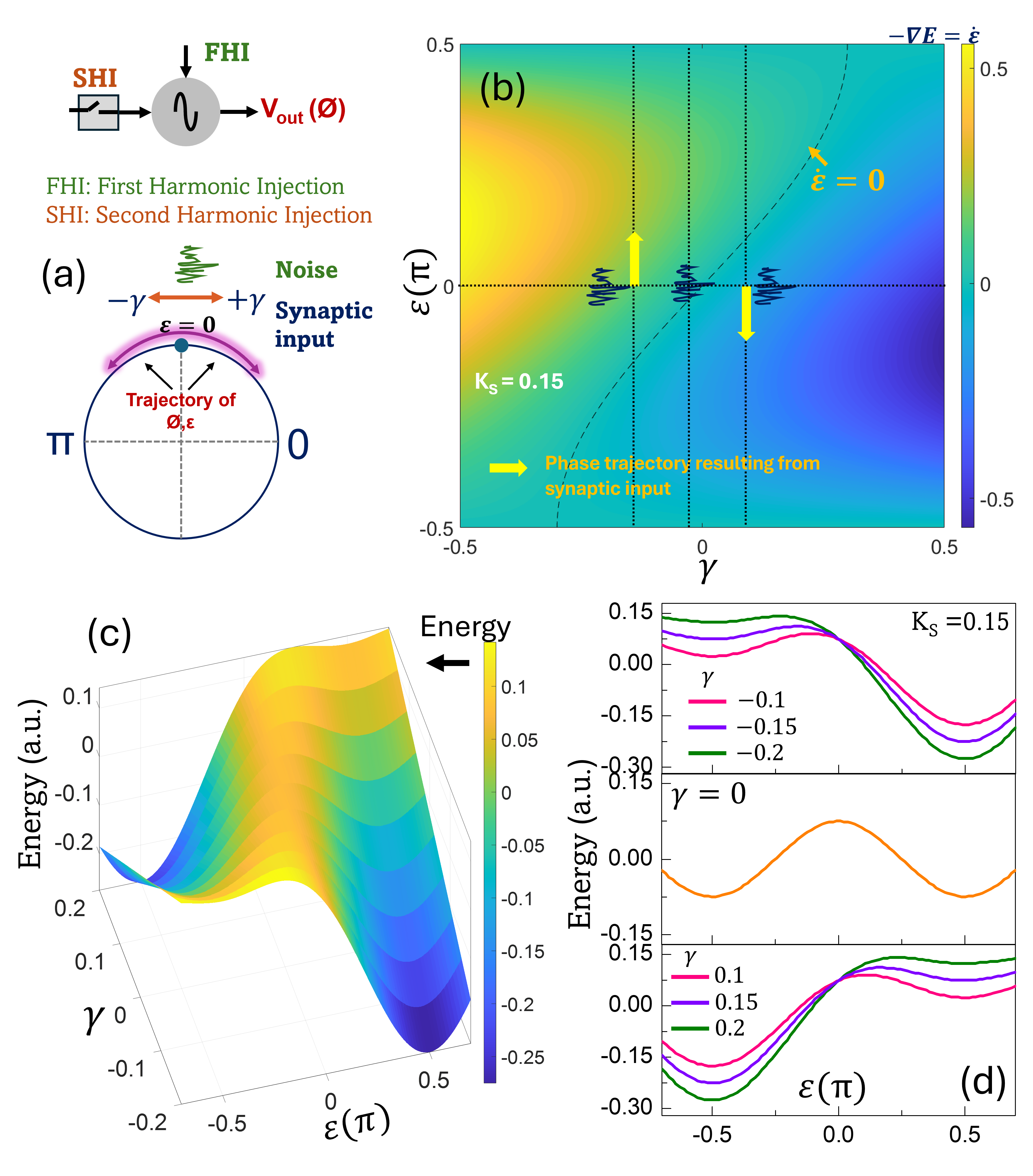
This diagram illustrates the effect of synaptic input on a system's energy landscape, likely related to neural dynamics or oscillatory networks. It depicts a system with first and second harmonic injections, a phase space representation of its dynamics, and a 3D visualization of its energy function. The diagram is divided into four sub-panels: (a) a schematic of the input signals, (b) a phase portrait, (c) a 3D energy landscape, and (d) cross-sectional energy profiles.
### Components/Axes
* **(a) Input Schematic:**
* Labels: "FHI" (First Harmonic Injection), "SHI" (Second Harmonic Injection), "V<sub>out</sub>(ø)", "Noise", "Synaptic input".
* Arrows indicate signal flow.
* **(b) Phase Portrait:**
* Axes: ε (vertical, ranging from -0.5 to 0.5), γ (horizontal, ranging from -0.5 to 0.5).
* Label: "-∇E = ε" at the top-right.
* Line: ε = 0 (dashed horizontal line).
* Arrows: Represent phase trajectories resulting from synaptic input.
* Parameter: K<sub>s</sub> = 0.15
* **(c) Energy Landscape:**
* Axes: γ (horizontal, ranging from -0.2 to 0.5), ε (π) (vertical, ranging from -0.25 to 0.1).
* Label: "Energy (a.u.)" with an arrow pointing upwards.
* **(d) Energy Profiles:**
* Axes: ε(π) (horizontal, ranging from -0.5 to 0.5), Energy (a.u.) (vertical, ranging from -0.3 to 0.15).
* Parameter: K<sub>s</sub> = 0.15
* Lines: Represent energy profiles for different values of γ (-0.1, -0.15, -0.2).
### Detailed Analysis or Content Details
**(a) Input Schematic:**
The schematic shows two input signals: First Harmonic Injection (FHI) and Second Harmonic Injection (SHI) feeding into an output signal V<sub>out</sub>(ø). Noise and synaptic input are also indicated as influencing the system.
**(b) Phase Portrait:**
The phase portrait displays the system's dynamics in the ε-γ plane. The dashed line ε = 0 divides the space. The arrows indicate trajectories influenced by synaptic input. The trajectories appear to converge towards the ε = 0 line, with some exhibiting oscillatory behavior. The parameter K<sub>s</sub> = 0.15 is noted.
**(c) Energy Landscape:**
The 3D plot shows the energy of the system as a function of γ and ε(π). The energy surface is complex, with a minimum around γ ≈ 0.2 and ε(π) ≈ -0.15. The color gradient indicates energy levels, with blue representing lower energy and yellow/green representing higher energy.
**(d) Energy Profiles:**
This panel presents cross-sectional energy profiles for different values of γ.
* **γ = -0.1:** The energy profile is approximately a parabola, with a minimum around ε(π) ≈ 0. Energy values range from approximately -0.2 to 0.05.
* **γ = -0.15:** The energy profile is shifted to the left, with a minimum around ε(π) ≈ -0.1. Energy values range from approximately -0.25 to 0.05.
* **γ = -0.2:** The energy profile is further shifted to the left, with a minimum around ε(π) ≈ -0.2. Energy values range from approximately -0.3 to 0.05.
The profiles demonstrate that the minimum energy state shifts with changes in γ.
### Key Observations
* The energy landscape in (c) is not symmetric, suggesting a directional bias in the system's dynamics.
* The energy profiles in (d) show a clear relationship between γ and the optimal ε(π) for minimizing energy. As γ decreases, the optimal ε(π) also decreases.
* The phase portrait in (b) suggests that synaptic input can stabilize the system around the ε = 0 line.
* The parameter K<sub>s</sub> = 0.15 appears to be a constant influencing the system's behavior.
### Interpretation
This diagram likely represents a model of a neural oscillator or a similar dynamical system. The FHI and SHI represent driving forces, while the synaptic input modulates the system's behavior. The energy landscape (c) provides a visualization of the system's stability and potential attractors. The minimum of the energy landscape corresponds to a stable state. The cross-sectional energy profiles (d) reveal how the stable state changes with variations in the synaptic input strength (γ).
The phase portrait (b) shows how synaptic input influences the system's trajectory in the ε-γ plane. The convergence of trajectories towards the ε = 0 line suggests that synaptic input can drive the system towards a specific state. The diagram as a whole suggests that the system can adapt its dynamics based on synaptic input, potentially enabling it to perform computations or maintain stable oscillations. The parameter K<sub>s</sub> likely represents a scaling factor or gain parameter influencing the overall system dynamics. The diagram is a theoretical exploration of the interplay between input signals, energy landscapes, and system dynamics, potentially relevant to understanding neural circuits or other oscillatory systems.