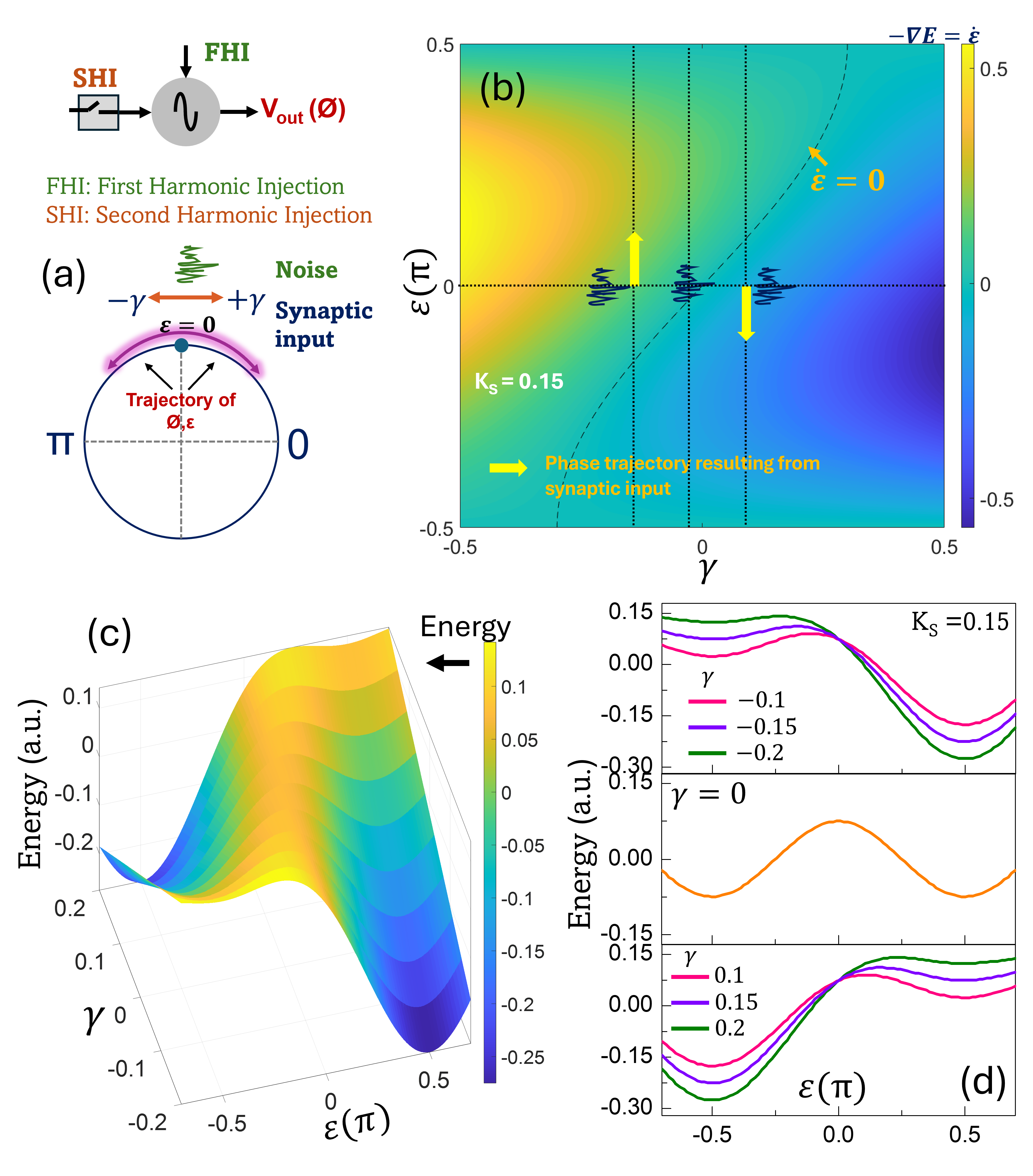
## Multi-Panel Scientific Diagram: Neuronal Dynamics and Energy Landscapes ### Overview The image presents a multi-panel scientific diagram analyzing neuronal dynamics through harmonic injections, phase trajectories, and energy landscapes. Key elements include: - First/Second Harmonic Injection (FHI/SHI) mechanisms - Phase-space trajectories with synaptic noise - Energy landscapes as functions of phase (ε) and gain (γ) - Stability analysis across parameter space ### Components/Axes #### Panel (a): Harmonic Injection Mechanism - **Diagram Elements**: - Circular trajectory labeled "Trajectory of Θ,ε" - Arrows indicating: - Noise: ±γ (orange) - Synaptic input: +γ (blue) - Labels: - FHI: First Harmonic Injection (green) - SHI: Second Harmonic Injection (orange) - Axes: Θ (horizontal), ε (vertical) #### Panel (b): Phase Trajectory Heatmap - **Axes**: - x-axis: γ (gain parameter, -0.5 to 0.5) - y-axis: ε(π) (phase, -0.5 to 0.5) - **Color Scale**: - Blue (-0.5) to Yellow (0.5) representing -∇E = ε - **Key Features**: - Vertical dashed line at γ = 0 - Yellow arrows marking: - ε = 0 (horizontal equilibrium) - -∇E = ε (diagonal equilibrium) - Ks = 0.15 (critical coupling parameter) #### Panel (c): 3D Energy Landscape - **Axes**: - x-axis: ε(π) (-0.5 to 0.5) - y-axis: γ (-0.2 to 0.2) - z-axis: Energy (a.u., -0.25 to 0.1) - **Color Gradient**: - Blue (low energy) to Yellow (high energy) - **Key Feature**: - Saddle-like structure with energy minima/maxima #### Panel (d): Energy vs Phase Curves - **Axes**: - x-axis: ε(π) (-0.5 to 0.5) - y-axis: Energy (a.u., -0.3 to 0.15) - **Data Series** (Ks = 0.15): - Orange: γ = 0 (baseline) - Red: γ = -0.1 (downward slope) - Purple: γ = -0.15 (steepest descent) - Green: γ = -0.2 (most negative slope) - Blue: γ = 0.1 (ascending slope) - Pink: γ = 0.15 (shallow ascent) - Green: γ = 0.2 (steepest ascent) ### Detailed Analysis #### Panel (a) - Circular trajectory shows phase-amplitude coupling - Noise (γ) modulates trajectory width - FHI/SHI labels suggest harmonic perturbation mechanisms #### Panel (b) - Phase trajectories cluster near: - ε = 0 (horizontal equilibrium) - -∇E = ε (diagonal stability boundary) - Ks = 0.15 indicates moderate coupling strength #### Panel (c) - Energy landscape reveals: - Double-well structure for γ < 0 - Monotonic increase for γ > 0 - Critical point at γ = 0, ε = 0 #### Panel (d) - Energy curves demonstrate: - γ < 0: Energy decreases with increasing ε - γ > 0: Energy increases with ε - Steeper slopes for |γ| > 0.15 ### Key Observations 1. **Bistability**: Panel (c) shows distinct energy minima for negative γ values 2. **Critical Coupling**: Ks = 0.15 appears in both (b) and (d), suggesting parameter consistency 3. **Slope Correlation**: Panel (d) confirms steeper energy gradients for |γ| > 0.15 4. **Equilibrium Points**: Panel (b) identifies two stable equilibria (ε=0 and -∇E=ε) ### Interpretation This diagram illustrates how synaptic noise (γ) and phase (ε) interact to shape neuronal energy landscapes. The FHI/SHI mechanism (a) likely represents input perturbations that drive the system toward different stability regimes. The heatmap (b) reveals how gain (γ) modulates phase trajectories, with Ks = 0.15 marking a critical coupling threshold. The 3D landscape (c) visualizes energy minima/maxima, while panel (d) quantifies how γ affects energy-phase relationships. Notably, negative γ values create bistable energy wells, suggesting potential for memory-like states in neuronal dynamics. The consistent Ks value across panels implies a unified parameter space for analyzing these interactions.