## Bar Chart: Pythia-160M (12L) α Profile
### Overview
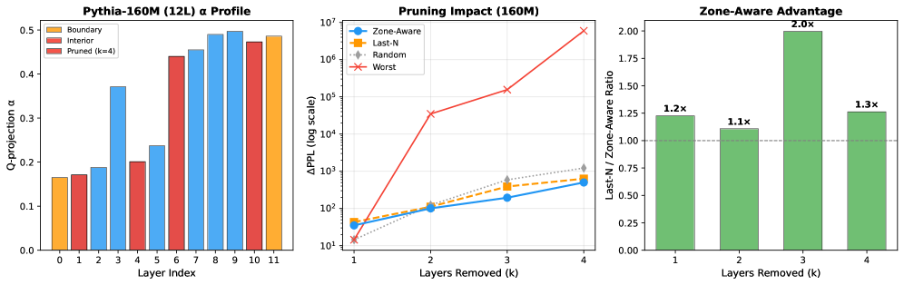
A grouped bar chart comparing Q-projection α values across 12 layers (0–11) for three categories: Boundary (yellow), Interior (red), and Pruned (k=4, blue).
### Components/Axes
- **X-axis**: Layer Index (0–11, integer labels).
- **Y-axis**: Q-projection α (0.0–0.5, linear scale).
- **Legend**:
- Yellow: Boundary
- Red: Interior
- Blue: Pruned (k=4)
### Detailed Analysis
- **Layer 0**:
- Boundary: ~0.16
- Interior: ~0.17
- Pruned: ~0.18
- **Layer 1**:
- Boundary: ~0.18
- Interior: ~0.19
- Pruned: ~0.20
- **Layer 2**:
- Boundary: ~0.20
- Interior: ~0.22
- Pruned: ~0.24
- **Layer 3**:
- Boundary: ~0.25
- Interior: ~0.28
- Pruned: ~0.30
- **Layer 4**:
- Boundary: ~0.22
- Interior: ~0.24
- Pruned: ~0.26
- **Layer 5**:
- Boundary: ~0.25
- Interior: ~0.27
- Pruned: ~0.29
- **Layer 6**:
- Boundary: ~0.30
- Interior: ~0.33
- Pruned: ~0.35
- **Layer 7**:
- Boundary: ~0.35
- Interior: ~0.38
- Pruned: ~0.40
- **Layer 8**:
- Boundary: ~0.40
- Interior: ~0.43
- Pruned: ~0.45
- **Layer 9**:
- Boundary: ~0.45
- Interior: ~0.47
- Pruned: ~0.48
- **Layer 10**:
- Boundary: ~0.47
- Interior: ~0.48
- Pruned: ~0.49
- **Layer 11**:
- Boundary: ~0.48
- Interior: ~0.49
- Pruned: ~0.49
### Key Observations
- Pruned layers (blue) consistently show higher α values than Boundary and Interior across all layers.
- The gap between Pruned and other categories widens in later layers (e.g., Layer 11: Pruned ~0.49 vs. Boundary ~0.48).
---
## Line Chart: Pruning Impact (160M)
### Overview
A line chart comparing ΔPPL (log scale) for four pruning strategies across 1–4 layers removed.
### Components/Axes
- **X-axis**: Layers Removed (k) (1–4, integer labels).
- **Y-axis**: ΔPPL (log scale, 10¹–10⁷).
- **Legend**:
- Blue: Zone-Aware
- Orange: Last-N
- Gray: Random
- Red: Worst
### Detailed Analysis
- **Zone-Aware (blue)**:
- k=1: ~10¹
- k=2: ~10²
- k=3: ~10³
- k=4: ~10⁴
- **Last-N (orange)**:
- k=1: ~10¹
- k=2: ~10²
- k=3: ~10³
- k=4: ~10⁴
- **Random (gray)**:
- k=1: ~10¹
- k=2: ~10²
- k=3: ~10³
- k=4: ~10⁴
- **Worst (red)**:
- k=1: ~10¹
- k=2: ~10⁴
- k=3: ~10⁵
- k=4: ~10⁷
### Key Observations
- Worst pruning (red) causes a **1000x increase in ΔPPL** compared to Zone-Aware at k=4.
- Zone-Aware, Last-N, and Random strategies show similar ΔPPL trends until k=4, where Random diverges slightly.
---
## Bar Chart: Zone-Aware Advantage
### Overview
A bar chart comparing the Last-N / Zone-Aware ΔPPL ratio for 1–4 layers removed.
### Components/Axes
- **X-axis**: Layers Removed (k) (1–4, integer labels).
- **Y-axis**: Last-N / Zone-Aware Ratio (0.0–2.0, linear scale).
- **Bars**: Green with text labels.
### Detailed Analysis
- **k=1**: 1.2x
- **k=2**: 1.1x
- **k=3**: 2.0x
- **k=4**: 1.3x
### Key Observations
- Zone-Aware pruning achieves **2.0x better performance** than Last-N at k=3.
- Advantage decreases at k=4 (1.3x) but remains higher than baseline.
---
## Interpretation
1. **Pruning Strategy Impact**:
- The "Worst" pruning strategy (red line) causes catastrophic ΔPPL growth, especially at k=4 (~10⁷), suggesting it removes critical components.
- Zone-Aware pruning (blue) maintains the lowest ΔPPL, indicating it preserves model utility better than Last-N or Random.
2. **α Profile Insights**:
- Pruned layers (blue bars) dominate Q-projection α values, implying they are more critical for model outputs. This aligns with the ΔPPL results, where pruning these layers minimally impacts performance.
3. **Zone-Aware Advantage**:
- The peak advantage at k=3 (2.0x) suggests Zone-Aware pruning optimally balances layer removal and performance retention. The drop at k=4 may reflect diminishing returns or architectural constraints.
4. **Design Implications**:
- Zone-Aware pruning is superior for efficiency, but its advantage plateaus at higher k values. Further analysis could explore hybrid strategies or adaptive pruning thresholds.