## Histogram: Sample Distributions
### Overview
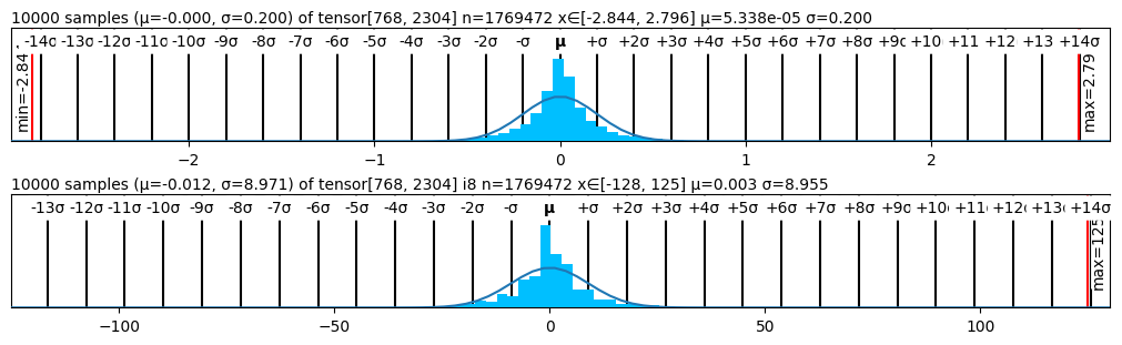
The image presents two histograms, each displaying the distribution of 10000 samples. The top histogram has a mean (μ) of approximately -0.000 and a standard deviation (σ) of 0.200, while the bottom histogram has a mean (μ) of approximately -0.012 and a standard deviation (σ) of 8.971. Both histograms show a roughly normal distribution centered around their respective means.
### Components/Axes
**Top Histogram:**
* **Title:** 10000 samples (μ=-0.000, σ=0.200) of tensor[768, 2304] n=1769472 x∈[-2.844, 2.796] μ=5.338e-05 σ=0.200
* **X-Axis:** Labeled with values from -2 to 2. Tick marks are also labeled with multiples of the standard deviation (σ) from -14σ to +14σ relative to the mean (μ).
* **Y-Axis:** (Implicit) Represents the frequency or count of samples within each bin.
* **Distribution:** The histogram bars are cyan. A blue curve, representing a normal distribution, is overlaid.
* **Min/Max:** A red line on the left indicates min = -2.84. A red line on the right indicates max = 2.79.
**Bottom Histogram:**
* **Title:** 10000 samples (μ=-0.012, σ=8.971) of tensor[768, 2304] i8 n=1769472 x∈[-128, 125] μ=0.003 σ=8.955
* **X-Axis:** Labeled with values from -100 to 100. Tick marks are also labeled with multiples of the standard deviation (σ) from -13σ to +14σ relative to the mean (μ).
* **Y-Axis:** (Implicit) Represents the frequency or count of samples within each bin.
* **Distribution:** The histogram bars are cyan. A blue curve, representing a normal distribution, is overlaid.
* **Min/Max:** A red line on the right indicates max = 125.
### Detailed Analysis
**Top Histogram:**
* The distribution is centered around 0, as indicated by the mean (μ ≈ -0.000).
* The spread of the data is relatively narrow, as indicated by the small standard deviation (σ = 0.200).
* The x-axis ranges from approximately -2.844 to 2.796.
* The minimum value is -2.84 and the maximum value is 2.79.
**Bottom Histogram:**
* The distribution is centered around 0, as indicated by the mean (μ ≈ -0.012).
* The spread of the data is much wider compared to the top histogram, as indicated by the larger standard deviation (σ = 8.971).
* The x-axis ranges from -128 to 125.
* The maximum value is 125.
### Key Observations
* Both histograms represent distributions of 10000 samples.
* The top histogram has a much smaller standard deviation compared to the bottom histogram, indicating a more concentrated distribution around the mean.
* The x-axis scales are significantly different between the two histograms, reflecting the different standard deviations.
### Interpretation
The two histograms visualize the distribution of two different sets of samples. The top histogram represents data with a small standard deviation, indicating that the values are clustered closely around the mean. The bottom histogram represents data with a much larger standard deviation, indicating that the values are more spread out. The titles provide additional information about the tensor shapes and sample sizes used to generate the histograms. The overlaid normal distribution curves provide a visual comparison of how well the data fits a normal distribution. The values of min and max are indicated by red lines.