## Histograms: Distribution of Samples
### Overview
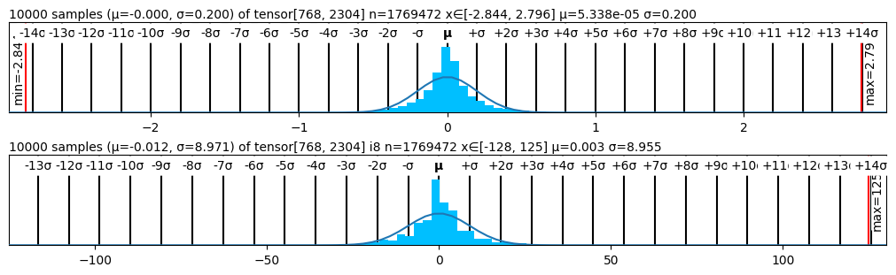
The image presents two histograms, each displaying the distribution of 10,000 samples. Each histogram is accompanied by statistical information regarding the mean (μ) and standard deviation (σ) of the samples. A fitted curve is overlaid on each histogram, likely representing a normal distribution.
### Components/Axes
Each histogram shares the following components:
* **X-axis:** Represents the sample values, ranging from approximately -140 to +140 in the top histogram and -130 to +130 in the bottom histogram. The axis is marked with tick labels at intervals of 10.
* **Y-axis:** Represents the frequency or count of samples within each bin. The Y-axis is not explicitly labeled, but is implied to be frequency.
* **Title:** Each histogram has a title indicating the number of samples (10000), the mean (μ) and standard deviation (σ) of the samples, the tensor size, and the range of the data.
* **Fitted Curve:** A blue curve is overlaid on each histogram, representing a fitted distribution (likely normal).
* **Vertical Lines:** Vertical lines are present at the mean (μ) and at ±1, ±2, ±3 standard deviations (σ) from the mean.
* **Min/Max Labels:** Labels indicating the minimum and maximum values of the data are present on the right side of each histogram.
**Specifics for each histogram:**
* **Top Histogram:**
* Title: "10000 samples (μ=-0.000, σ=0.200) of tensor[768, 2304] n=1769472 x∈[-2.844, 2.796] μ=5.338e-05 σ=0.200"
* Min: -2.844
* Max: 2.796
* **Bottom Histogram:**
* Title: "10000 samples (μ=-0.012, σ=8.971) of tensor[768, 2304] n=1769472 x∈[-128, 125] μ=0.003 σ=8.955"
* Min: -128
* Max: 125
### Detailed Analysis or Content Details
**Top Histogram:**
* The distribution is approximately normal, centered around 0.
* The fitted blue curve closely follows the histogram bars.
* The histogram is relatively narrow, indicating a small standard deviation (σ = 0.200).
* The data ranges from approximately -2.8 to 2.8.
* The frequency is highest around 0, and decreases symmetrically as you move away from 0.
**Bottom Histogram:**
* The distribution is also approximately normal, but is much wider than the top histogram.
* The fitted blue curve follows the histogram bars, but with more deviation than the top histogram.
* The standard deviation is significantly larger (σ = 8.971).
* The data ranges from approximately -128 to 125.
* The frequency is highest around 0, and decreases as you move away from 0.
### Key Observations
* The two histograms represent distributions with very different scales. The top histogram has a much smaller range and standard deviation than the bottom histogram.
* Both distributions appear to be centered around 0, although the bottom histogram's mean is slightly negative (-0.012).
* The wider spread of the bottom histogram suggests greater variability in the data.
* The tensor size is the same for both histograms.
### Interpretation
The image demonstrates two different distributions of samples. The top histogram represents a distribution with low variance, tightly clustered around zero. This could represent a highly controlled or precise process. The bottom histogram, in contrast, represents a distribution with high variance, spread over a much wider range. This could represent a more noisy or unpredictable process.
The statistical information provided (μ and σ) quantifies these differences. The small standard deviation of the top histogram (0.200) confirms its narrow spread, while the large standard deviation of the bottom histogram (8.971) confirms its wide spread.
The fitted curves suggest that both distributions can be reasonably approximated by a normal distribution, despite their different scales. The tensor size indicates that the data is likely from a multi-dimensional array, and the 'n' value suggests the total number of data points used in the analysis. The x∈[...] notation indicates the range of the data.