# Technical Document Extraction: Histogram Analysis
## Overview
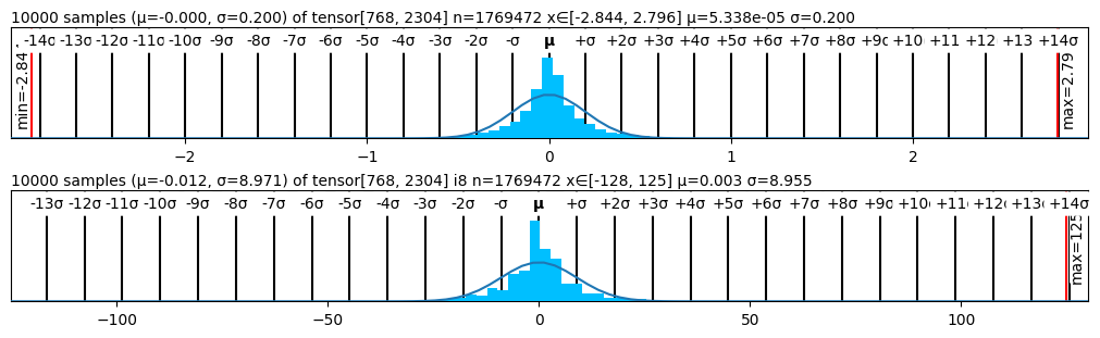
The image contains two histograms with overlaid normal distribution curves, representing statistical distributions of sampled data. Both histograms include axis labels, legends, and annotations for statistical parameters.
---
### **Top Histogram**
#### **Title & Parameters**
- **Title**: `10000 samples (μ=-0.000, σ=0.200) of tensor[768, 2304] n=1769472 x∈[-2.844, 2.796] μ=5.338e-05 σ=0.200`
- **Statistical Summary**:
- **Minimum Value**: `-2.84` (marked with red vertical line on the left)
- **Maximum Value**: `2.796` (marked with red vertical line on the right)
- **Mean (μ)**: `5.338e-05`
- **Standard Deviation (σ)**: `0.200`
- **Sample Count (n)**: `1769472`
- **Range**: `x ∈ [-2.844, 2.796]`
#### **Axis Labels**
- **X-Axis**: Labeled with multiples of σ (e.g., `-14σ`, `-13σ`, ..., `+14σ`), spanning from `-2.84` to `2.796`.
- **Y-Axis**: Labeled `10000 samples`.
#### **Legend**
- **Location**: Right side of the histogram.
- **Content**: Blue curve labeled `Normal Distribution`.
#### **Visual Trends**
- The histogram follows a bell-shaped curve, peaking near `μ = 0` (centered at `0` due to symmetry).
- The distribution is tightly clustered around the mean, with most data points within `±3σ` (i.e., `[-0.6, 0.6]`).
- The red vertical lines at `min = -2.84` and `max = 2.796` indicate the extreme values of the dataset.
---
### **Bottom Histogram**
#### **Title & Parameters**
- **Title**: `10000 samples (μ=0.0012, σ=8.971) of tensor[768, 2304] i8 n=1769472 x∈[-128, 125] μ=0.0003 σ=8.955`
- **Statistical Summary**:
- **Minimum Value**: `-128` (marked with red vertical line on the left)
- **Maximum Value**: `125` (marked with red vertical line on the right)
- **Mean (μ)**: `0.0003`
- **Standard Deviation (σ)**: `8.955`
- **Sample Count (n)**: `1769472`
- **Range**: `x ∈ [-128, 125]`
#### **Axis Labels**
- **X-Axis**: Labeled with multiples of σ (e.g., `-13σ`, `-12σ`, ..., `+14σ`), spanning from `-128` to `125`.
- **Y-Axis**: Labeled `10000 samples`.
#### **Legend**
- **Location**: Right side of the histogram.
- **Content**: Blue curve labeled `Normal Distribution`.
#### **Visual Trends**
- The histogram also follows a bell-shaped curve but is significantly wider than the top histogram, reflecting a larger standard deviation (`σ = 8.955`).
- The distribution is centered near `μ = 0.0003`, with most data points spread across `±3σ` (i.e., `[-26.865, 26.865]`).
- The red vertical lines at `min = -128` and `max = 125` indicate the extreme values of the dataset.
---
### **Key Observations**
1. **Normal Distribution Fit**: Both histograms closely approximate a normal distribution, as evidenced by the overlaid blue curve.
2. **Scale Differences**:
- The top histogram has a narrow range (`[-2.844, 2.796]`) and small σ (`0.200`), indicating low variability.
- The bottom histogram has a wide range (`[-128, 125]`) and large σ (`8.955`), indicating high variability.
3. **Legend Consistency**: The blue curve in both histograms matches the legend label `Normal Distribution`, confirming the statistical model used.
4. **Axis Markers**: X-axis labels are spaced at integer multiples of σ, providing a standardized reference for data spread.
---
### **Conclusion**
The histograms illustrate two distinct normal distributions with differing scales of variability. The top histogram represents a tightly clustered dataset, while the bottom histogram shows a dataset with significant spread. Both include explicit annotations for statistical parameters and data ranges.