## 3D Surface Plot: Saddle Surface over a Square Domain
### Overview
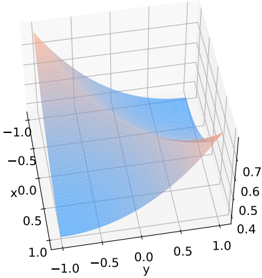
The image displays a three-dimensional surface plot rendered within a cubic bounding box. The plot visualizes a mathematical function over a square domain in the x-y plane. The surface exhibits a characteristic saddle shape, with its curvature changing direction along different axes. The visualization uses a color gradient to represent the height (z-value) of the surface.
### Components/Axes
* **Plot Type:** 3D Surface Plot.
* **Bounding Box:** A wireframe cube defines the plotting volume.
* **Axes:**
* **X-axis:** Located on the left side, running vertically. Label: `x`. Scale: Linear, ranging from `-1.0` at the top to `1.0` at the bottom. Major tick marks at `-1.0`, `-0.5`, `0.0`, `0.5`, `1.0`.
* **Y-axis:** Located at the bottom front, running horizontally. Label: `y`. Scale: Linear, ranging from `-1.0` on the left to `1.0` on the right. Major tick marks at `-1.0`, `-0.5`, `0.0`, `0.5`, `1.0`.
* **Z-axis (Vertical):** Located on the right side. No explicit label, but represents the function value. Scale: Linear, ranging from approximately `0.4` at the bottom to `0.7` at the top. Major tick marks visible at `0.4`, `0.5`, `0.6`, `0.7`.
* **Surface:** A continuous, smooth surface spanning the domain where `x` and `y` are both between `-1.0` and `1.0`.
* **Color Mapping:** The surface uses a diverging color gradient. Lower z-values (near 0.4) are colored in shades of blue. Higher z-values (near 0.7) are colored in shades of red/orange. The midpoint of the color scale appears to be a neutral grayish tone.
* **Legend:** There is no separate legend box. The color-to-value mapping is implied by the gradient on the surface itself and the z-axis tick labels.
### Detailed Analysis
* **Surface Geometry:** The surface is a classic saddle shape (hyperbolic paraboloid). It curves upward along one diagonal direction and downward along the other.
* **High Points:** The highest points (red/orange) are located at the four corners of the domain: `(x=-1, y=-1)`, `(x=-1, y=1)`, `(x=1, y=-1)`, and `(x=1, y=1)`. The z-value at these corners is approximately `0.7`.
* **Low Points:** The lowest points (blue) are located at the midpoints of the four edges of the domain: `(x=0, y=-1)`, `(x=0, y=1)`, `(x=-1, y=0)`, and `(x=1, y=0)`. The z-value at these edge midpoints is approximately `0.4`.
* **Center Point:** The center of the domain `(x=0, y=0)` is a saddle point. The surface is relatively flat here, with a z-value approximately midway between the high and low extremes, estimated at `0.55`. The color at the center is a transitional gray-blue.
* **Trend Verification:**
* Moving from the center `(0,0)` towards any corner (e.g., `(1,1)`), the surface slopes **upward**, and the color shifts from gray-blue to red.
* Moving from the center `(0,0)` towards the midpoint of any edge (e.g., `(0,1)`), the surface slopes **downward**, and the color shifts from gray-blue to deeper blue.
* **Spatial Grounding:** The z-axis is positioned on the right side of the bounding box. The x-axis label is on the left vertical edge. The y-axis label is on the bottom front edge. The surface fills the entire plotted volume.
### Key Observations
1. **Symmetry:** The surface is symmetric about both the `x=0` and `y=0` planes. The pattern of highs and lows is mirrored across these axes.
2. **Color-Value Correlation:** The color gradient provides a clear visual cue for height. Red/orange consistently marks the highest regions, while blue marks the lowest.
3. **Saddle Point:** The point at `(0,0)` is a critical point where the surface has zero slope in all directions but is not an extremum (it's a minimax point).
4. **Domain Boundary:** The surface is clipped exactly at the boundaries `x = ±1` and `y = ±1`, forming a square "patch" of the mathematical surface.
### Interpretation
This plot visualizes a function of the form `z = f(x, y)`. The specific shape strongly suggests the function is `z = 0.55 + 0.15 * (x² - y²)` or a similar quadratic form like `z = 0.55 + 0.15 * x*y` (rotated 45 degrees). The data demonstrates a **saddle surface**, which is fundamental in multivariable calculus and optimization theory.
* **What it represents:** It shows a relationship where the output `z` increases when moving away from the center along one axis (e.g., `x`) but decreases when moving away along the other axis (e.g., `y`). This is characteristic of functions with a **minimax** or **saddle point**.
* **Why it matters:** Such surfaces appear in various scientific contexts:
* **Optimization:** The saddle point `(0,0)` represents a critical point that is neither a local maximum nor a local minimum, posing challenges for gradient-based optimization algorithms.
* **Physics:** Can model potential energy surfaces in systems with competing forces, or the shape of a physical saddle.
* **Economics:** Might represent a utility or production function with trade-offs between two inputs.
* **Notable Anomaly:** There are no anomalies; the surface is a smooth, mathematically ideal representation. The key takeaway is the clear visual distinction between the rising diagonals (toward corners) and falling diagonals (toward edge midpoints), perfectly encoded in both geometry and color.