## Directed Acyclic Graph (Causal Diagram): Instrumental Variable Model
### Overview
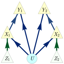
The image displays a directed acyclic graph (DAG), a type of diagram used in causal inference and statistics to represent hypothesized relationships between variables. The diagram illustrates a classic instrumental variable (IV) setup with two parallel systems, likely representing two distinct groups, time points, or measurement instances.
### Components/Axes
The diagram consists of seven labeled nodes (variables) and directed edges (arrows) indicating causal pathways.
**Nodes (Variables):**
* **U**: A central, circular node at the bottom center. It is colored light blue.
* **Z₁**: A triangular node at the bottom-left. It is colored light yellow.
* **Z₂**: A triangular node at the bottom-right. It is colored light yellow.
* **X₁**: A triangular node in the middle-left, above Z₁. It is colored light yellow.
* **X₂**: A triangular node in the middle-right, above Z₂. It is colored light yellow.
* **Y₁**: A triangular node at the top-left, above X₁. It is colored light yellow.
* **Y₂**: A triangular node at the top-right, above X₂. It is colored light yellow.
**Edges (Arrows):**
The arrows are colored, indicating different types of relationships. There is no explicit legend, but the color coding is consistent.
* **Green Arrows**: Two arrows originate from the Z nodes.
* From **Z₁** to **X₁**.
* From **Z₂** to **X₂**.
* **Blue Arrows**: Multiple arrows originate from U and the X nodes.
* From **U** to **X₁**.
* From **U** to **X₂**.
* From **U** to **Y₁**.
* From **U** to **Y₂**.
* From **X₁** to **Y₁**.
* From **X₂** to **Y₂**.
### Detailed Analysis
The diagram is structured hierarchically and symmetrically.
1. **Spatial Layout**: The graph has a clear top (Y variables), middle (X variables), and bottom (Z variables and U). The central node **U** is positioned at the bottom center, acting as a common source.
2. **Flow and Relationships**:
* **Instrumental Variables (Z₁, Z₂)**: These are exogenous variables that influence the treatment/exposure variables (X₁, X₂) but have no direct path to the outcome variables (Y₁, Y₂). This is shown by the green arrows pointing only to the X nodes.
* **Treatment/Exposure Variables (X₁, X₂)**: These are influenced by both their respective instrumental variable (Z) and the unobserved confounder (U). They, in turn, influence their respective outcome variable (Y).
* **Outcome Variables (Y₁, Y₂)**: These are influenced by their corresponding treatment variable (X) and directly by the unobserved confounder (U).
* **Unobserved Confounder (U)**: This central node has direct blue arrows pointing to all four X and Y variables, representing a common cause that confounds the relationship between X and Y.
### Key Observations
* **Symmetry**: The diagram is perfectly symmetrical around the vertical axis passing through node U. The left system (Z₁, X₁, Y₁) is a mirror image of the right system (Z₂, X₂, Y₂).
* **Color Coding**: The arrow colors are used systematically. Green denotes the path from instrument to treatment. Blue denotes all other causal paths, including the confounding paths from U and the direct treatment-to-outcome effect.
* **Absence of Direct Z→Y Path**: A critical feature for an instrumental variable is the absence of a direct arrow from Z to Y. This diagram correctly omits such a path for both Z₁ and Z₂.
* **Common Confounder**: The node **U** is connected to all other endogenous variables (X and Y), visually representing the core problem of omitted variable bias that instrumental variable analysis aims to address.
### Interpretation
This diagram is a formal representation of an **Instrumental Variable (IV) model**, likely for a two-sample or two-period setting. It visually encodes the key assumptions required for IV estimation:
1. **Relevance**: The instrument (Z) must affect the treatment (X). This is shown by the green arrows (Z₁→X₁, Z₂→X₂).
2. **Exclusion Restriction**: The instrument (Z) must affect the outcome (Y) *only* through the treatment (X). This is satisfied by the absence of a direct Z→Y arrow.
3. **Independence/Exchangeability**: The instrument (Z) must not share common causes with the outcome (Y). This is implied by Z having no incoming arrows from U or elsewhere.
The presence of **U** with arrows to both X and Y illustrates the **endogeneity problem**: the observed correlation between X and Y is biased because U influences both. The IV strategy uses the exogenous variation introduced by Z (which is not affected by U) to isolate the causal effect of X on Y.
The dual structure (subscripts 1 and 2) could represent several scenarios:
* **Two different instruments** (Z₁ and Z₂) for the same treatment-outcome relationship, allowing for overidentification tests.
* **Data from two different populations or time periods**, where the same causal structure is assumed to hold.
* A **mediation or structural equation model** where the relationships are being studied across two related contexts.
In essence, this diagram is a technical blueprint for a statistical analysis plan aimed at estimating a causal effect in the presence of unmeasured confounding.