## Combined Chart: Error vs. #particles and WCET vs. #particles
### Overview
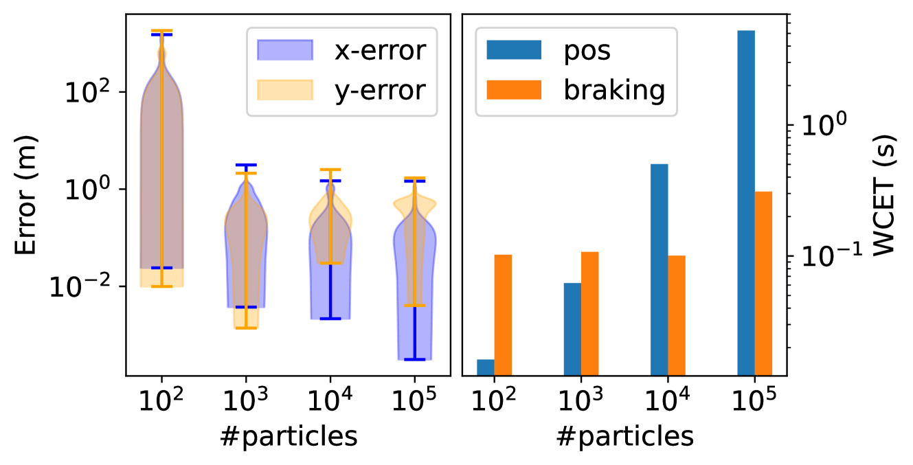
The image presents two charts side-by-side. The left chart is a violin plot showing the distribution of x-error and y-error as a function of the number of particles. The right chart is a bar plot showing the Worst-Case Execution Time (WCET) for 'pos' and 'braking' as a function of the number of particles. Both charts share the same x-axis: '#particles'. Both charts use a log scale for both axes.
### Components/Axes
**Left Chart (Error vs. #particles):**
* **Y-axis:** "Error (m)" - Logarithmic scale with markers at 10<sup>-2</sup>, 10<sup>0</sup>, and 10<sup>2</sup>.
* **X-axis:** "#particles" - Logarithmic scale with markers at 10<sup>2</sup>, 10<sup>3</sup>, 10<sup>4</sup>, and 10<sup>5</sup>.
* **Legend (Top-Right):**
* "x-error" - Light Blue
* "y-error" - Light Orange
**Right Chart (WCET vs. #particles):**
* **Y-axis:** "WCET (s)" - Logarithmic scale with markers at 10<sup>-1</sup> and 10<sup>0</sup>.
* **X-axis:** "#particles" - Logarithmic scale with markers at 10<sup>2</sup>, 10<sup>3</sup>, 10<sup>4</sup>, and 10<sup>5</sup>.
* **Legend (Top-Left):**
* "pos" - Dark Blue
* "braking" - Orange
### Detailed Analysis
**Left Chart (Error vs. #particles):**
* **x-error (Light Blue):**
* At 10<sup>2</sup> particles: The distribution is centered around 10<sup>1</sup> m, with a wide spread.
* At 10<sup>3</sup> particles: The distribution is centered around 10<sup>-1</sup> m, with a smaller spread.
* At 10<sup>4</sup> particles: The distribution is centered around 10<sup>-1</sup> m, with a smaller spread.
* At 10<sup>5</sup> particles: The distribution is centered around 10<sup>-1</sup> m, with a smaller spread.
* Trend: The x-error decreases significantly as the number of particles increases from 10<sup>2</sup> to 10<sup>3</sup>, then plateaus.
* **y-error (Light Orange):**
* At 10<sup>2</sup> particles: The distribution is centered around 10<sup>-2</sup> m, with a wide spread.
* At 10<sup>3</sup> particles: The distribution is centered around 10<sup>-2</sup> m, with a smaller spread.
* At 10<sup>4</sup> particles: The distribution is centered around 10<sup>-1</sup> m, with a smaller spread.
* At 10<sup>5</sup> particles: The distribution is centered around 10<sup>-1</sup> m, with a smaller spread.
* Trend: The y-error remains relatively constant as the number of particles increases, with a slight increase between 10<sup>3</sup> and 10<sup>4</sup>.
**Right Chart (WCET vs. #particles):**
* **pos (Dark Blue):**
* At 10<sup>2</sup> particles: WCET is approximately 0.02 s.
* At 10<sup>3</sup> particles: WCET is approximately 0.2 s.
* At 10<sup>4</sup> particles: WCET is approximately 0.6 s.
* At 10<sup>5</sup> particles: WCET is approximately 2 s.
* Trend: The WCET for 'pos' increases significantly as the number of particles increases.
* **braking (Orange):**
* At 10<sup>2</sup> particles: WCET is approximately 0.08 s.
* At 10<sup>3</sup> particles: WCET is approximately 0.15 s.
* At 10<sup>4</sup> particles: WCET is approximately 0.2 s.
* At 10<sup>5</sup> particles: WCET is approximately 0.4 s.
* Trend: The WCET for 'braking' increases as the number of particles increases, but not as dramatically as 'pos'.
### Key Observations
* Increasing the number of particles significantly reduces the x-error, especially between 10<sup>2</sup> and 10<sup>3</sup> particles.
* The y-error is less sensitive to the number of particles.
* The WCET for both 'pos' and 'braking' increases with the number of particles, but 'pos' is more affected.
* At 10^5 particles, the WCET for 'pos' is significantly higher than 'braking'.
### Interpretation
The data suggests that increasing the number of particles improves the accuracy of the 'x' position estimate, with diminishing returns beyond 10<sup>3</sup> particles. The 'y' position estimate is less affected by the number of particles. However, increasing the number of particles increases the computational cost, as reflected in the WCET. The 'pos' operation is more computationally expensive than 'braking' and its cost increases more rapidly with the number of particles. This information is useful for optimizing the particle filter algorithm, balancing accuracy and computational cost.