## 3D Surface Plots: Twisting Surfaces ### Overview The image contains two 3D surface plots, each depicting a series of twisting surfaces. The plots share similar axes and scales but offer different perspectives on the same or related data. The surfaces are represented by multiple colored lines, creating a visual effect of twisting or spiraling. ### Components/Axes Both plots share the following characteristics: * **Axes:** Each plot has three axes labeled X, Y, and Z. * **X-Axis:** The X-axis ranges from approximately -0.2 to 1.5. * **Y-Axis:** The Y-axis ranges from approximately -0.2 to 1.2. * **Z-Axis:** The Z-axis ranges from approximately -0.2 to 1.2. * **Gridlines:** Both plots have gridlines along each axis to aid in visualization. * **Surfaces:** Multiple colored lines represent the surfaces. The colors vary, but there is no explicit legend. ### Detailed Analysis **Left Plot:** * **Orientation:** The plot is oriented such that the viewer sees the surfaces twisting around a central point. * **Surface Shape:** The surfaces appear to start as a flat plane, twist inward towards the center, and then expand outward again, creating an hourglass-like shape. * **Color Variation:** The surfaces are represented by a range of colors, including blues, greens, yellows, oranges, and reds. The colors seem to be assigned sequentially to each surface. * **X-Y Plane:** The surfaces appear to be defined on a grid in the X-Y plane. **Right Plot:** * **Orientation:** The plot is oriented to show a side view of the twisting surfaces. * **Surface Shape:** From this perspective, the surfaces appear to start as a flat plane, twist upwards and to the side, and then flatten out again at the top. * **Color Variation:** Similar to the left plot, the surfaces are represented by a range of colors. * **X-Y Plane:** The surfaces appear to be defined on a grid in the X-Y plane. ### Key Observations * **Twisting Behavior:** Both plots clearly show the twisting nature of the surfaces. * **Symmetry:** The left plot suggests a degree of symmetry around the Z-axis. * **Perspective:** The two plots provide complementary perspectives, aiding in understanding the 3D shape of the surfaces. ### Interpretation The plots visualize a set of surfaces that undergo a twisting transformation. The left plot emphasizes the overall shape and symmetry, while the right plot highlights the twisting motion from a side view. The absence of a legend makes it difficult to determine the exact meaning of the different colors, but they likely represent different parameters or iterations of the twisting process. The data suggests a continuous transformation of a surface from a flat plane to a twisted shape and back to a flat plane. The plots are useful for understanding the spatial characteristics of this transformation.

\n ## 3D Surface Plots: Torus-like Structures ### Overview The image presents two 3D surface plots, both depicting a torus-like structure. The plots are visually similar, differing primarily in the orientation and color scheme used to represent the surface. Both plots utilize a Cartesian coordinate system (X, Y, Z) to define the spatial arrangement of the structure. The plots do not contain explicit data tables or numerical values, but rather visualize a continuous surface. ### Components/Axes Both plots share the following components: * **Axes:** * X-axis: Ranges approximately from -0.2 to 1.4 (right plot) and 0.0 to 1.5 (left plot). * Y-axis: Ranges approximately from -0.2 to 0.2 (right plot) and 0.0 to 1.2 (left plot). * Z-axis: Ranges approximately from 0.0 to 1.2 in both plots. * **Coordinate System:** Cartesian (X, Y, Z). * **Surface:** A torus-like shape, with a central hole. * **Coloring:** The surface is colored using a gradient of colors, which appears to represent the height or value of the surface at each point. ### Detailed Analysis or Content Details **Left Plot:** * The torus is oriented such that the hole is roughly aligned with the Y-axis. * The color gradient transitions from shades of red and orange (lower Z values) to purple and blue (higher Z values). * The X-axis extends from approximately 0.0 to 1.5. * The Y-axis extends from approximately 0.0 to 1.2. * The Z-axis extends from approximately 0.0 to 1.2. **Right Plot:** * The torus is rotated compared to the left plot, with the hole oriented more diagonally. * The color gradient is more diverse, including greens, yellows, and blues. * The X-axis extends from approximately -0.2 to 1.4. * The Y-axis extends from approximately -0.2 to 0.2. * The Z-axis extends from approximately 0.0 to 1.2. Both plots show a continuous surface with no sharp edges or discontinuities. The color variations suggest a smooth change in the surface's height or value. ### Key Observations * The two plots represent the same underlying torus-like structure, but viewed from different angles and with different color schemes. * The color gradients are used to visually represent the surface's height or value, with warmer colors generally indicating lower values and cooler colors indicating higher values. * The plots do not provide specific numerical data points, but rather a visual representation of a continuous surface. ### Interpretation The image demonstrates a visualization of a 3D torus-like surface. The use of color gradients allows for a quick understanding of the surface's shape and height variations. The two different orientations suggest an exploration of the structure from multiple viewpoints. The absence of explicit data points indicates that the image is intended to convey a general understanding of the shape rather than precise numerical values. The plots could represent a mathematical function, a physical object, or a simulation result. Without additional context, it is difficult to determine the specific meaning or application of the visualization. The plots are likely generated from a parametric equation defining the torus shape. The different color schemes could be used to highlight different features of the surface or to improve visual clarity.

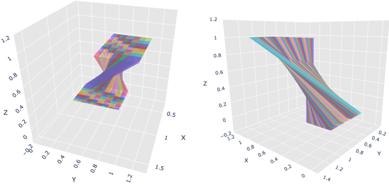
## 3D Surface Plots: Dual-Orientation Visualization ### Overview The image displays two separate 3D surface plots positioned side-by-side. Both plots visualize a complex, twisted surface within a 3D coordinate system, but from different camera angles and with distinct surface patterning. The left plot features a checkered or tiled pattern, while the right plot features a striped pattern. The surfaces appear to represent the same or a very similar mathematical function or dataset. ### Components/Axes **Left Plot (Checkered Pattern):** * **Axes:** Three orthogonal axes labeled X, Y, and Z. * **X-Axis:** Located on the right side of the plot's floor. Ticks and labels visible: `0.5`, `1`, `1.5`. The axis extends from approximately 0 to 1.5. * **Y-Axis:** Located on the front-left side of the plot's floor. Ticks and labels visible: `0`, `0.2`, `0.4`, `0.6`, `0.8`, `1`, `1.2`. The axis extends from approximately 0 to 1.2. * **Z-Axis:** The vertical axis on the left. Ticks and labels visible: `0`, `0.2`, `0.4`, `0.6`, `0.8`, `1`, `1.2`. The axis extends from approximately 0 to 1.2. * **Surface:** A 3D surface with a complex, saddle-like twist. It is colored with a multi-colored checkered pattern (tiles of blue, purple, pink, yellow, green). The pattern appears to be mapped onto the surface geometry. **Right Plot (Striped Pattern):** * **Axes:** Three orthogonal axes labeled X, Y, and Z. * **X-Axis:** Located on the front-left side of the plot's floor. Ticks and labels visible: `0`, `0.2`, `0.4`, `0.6`, `0.8`, `1`, `1.2`, `1.4`. The axis extends from approximately 0 to 1.4. * **Y-Axis:** Located on the right side of the plot's floor. Ticks and labels visible: `0`, `0.2`, `0.4`, `0.6`, `0.8`, `1`, `1.2`. The axis extends from approximately 0 to 1.2. * **Z-Axis:** The vertical axis on the left. Ticks and labels visible: `0`, `0.2`, `0.4`, `0.6`, `0.8`, `1`, `1.2`. The axis extends from approximately 0 to 1.2. * **Surface:** A 3D surface with a similar twisted geometry to the left plot, appearing as a ribbon or folded plane. It is colored with a multi-colored striped pattern (stripes of cyan, purple, pink, yellow, green). The stripes run along the length of the surface. **General Notes:** * **Legend:** No explicit legend is present in either plot. The color patterns (checkers vs. stripes) are the primary visual differentiators. * **Grid:** Both plots have a light gray grid on the "floor" (XY-plane) and the back walls (XZ and YZ planes) to aid in spatial orientation. * **Background:** The background of both plots is a uniform light gray. ### Detailed Analysis **Left Plot (Checkered):** * **Trend/Shape:** The surface starts at a low Z-value near the origin (X≈0, Y≈0), rises to a peak or ridge, then descends into a valley before rising again towards the far corner (X≈1.5, Y≈1.2). The overall shape resembles a hyperbolic paraboloid or a saddle point that has been twisted. * **Data Points (Approximate):** * Minimum Z: ~0.2, located near (X=0.2, Y=0.2). * Maximum Z: ~1.1, located near (X=1.0, Y=1.0). * The surface appears to be defined over the domain X ∈ [0, 1.5], Y ∈ [0, 1.2]. **Right Plot (Striped):** * **Trend/Shape:** The surface is viewed from a different angle, making the twist more apparent as a diagonal fold. It appears to descend from a high Z-value at the back-left (low X, high Y) to a low Z-value at the front-right (high X, low Y). The striped pattern emphasizes the flow and curvature along the surface. * **Data Points (Approximate):** * High Z-point: ~1.0, located near (X=0, Y=1.2). * Low Z-point: ~0.2, located near (X=1.4, Y=0). * The surface appears to be defined over the domain X ∈ [0, 1.4], Y ∈ [0, 1.2]. ### Key Observations 1. **Dual Representation:** The core observation is the visualization of the same (or very similar) 3D surface geometry using two different texture mappings: checkered and striped. 2. **Viewpoint Dependency:** The two plots are rendered from significantly different camera perspectives. The left plot offers a more "corner-on" view, while the right plot offers a more "side-on" view, highlighting different aspects of the surface's topology. 3. **Pattern Function:** The patterns are not indicative of different data series but are likely applied to enhance the perception of the surface's 3D shape, curvature, and orientation. The checkered pattern helps visualize local deformation, while the striped pattern emphasizes global flow. 4. **Axis Range Discrepancy:** The X-axis range differs slightly between the plots (0-1.5 vs. 0-1.4), which could be due to the viewing angle cropping the data or a slight difference in the plotted domain. ### Interpretation This image is a technical visualization, likely generated by mathematical software (e.g., MATLAB, Python's Matplotlib, Mathematica) to explore or present the properties of a 3D scalar field or parametric surface. * **What it Demonstrates:** The plots show a non-linear, twisted surface where the Z-value is a function of X and Y. The saddle-like shape suggests the function has a critical point (like a minimax point) within the domain. The use of different patterns and views is a common technique in data visualization to aid human depth perception and understanding of complex 3D forms on a 2D screen. * **Relationship Between Elements:** The axes provide the coordinate frame. The grid lines anchor the surface in that frame. The color patterns are mapped onto the surface geometry to reveal its contours. The two plots together provide a more complete mental model of the surface than a single view could. * **Notable Anomalies:** There are no apparent data anomalies, as this appears to be a smooth, continuous mathematical surface. The primary "anomaly" for a viewer is the intentional use of two distinct, non-standard color mappings (checkers and stripes) instead of a continuous colormap, which is a deliberate pedagogical or presentational choice to highlight surface geometry over scalar value. * **Potential Context:** Such visualizations are used in fields like multivariate calculus, optimization theory, computer graphics (for testing texture mapping), physics (for representing potential fields), or engineering (for stress/strain surfaces). The specific function being plotted is not labeled, but its characteristics (bounded, smooth, twisted) are clearly communicated.

## 3D Surface Plots: Comparative Analysis ### Overview The image contains two side-by-side 3D surface plots with distinct geometric configurations. Both plots use a color gradient (purple to green) to represent surface elevation or a related parameter. The left plot exhibits a saddle-shaped surface with a central peak, while the right plot displays a helical/spiral structure descending diagonally across the plot. ### Components/Axes **Left Plot:** - **X-axis**: Labeled "X", range [-0.2, 1.5], increments of 0.2 - **Y-axis**: Labeled "Y", range [0, 1.2], increments of 0.2 - **Z-axis**: Labeled "Z", range [0, 1.2], increments of 0.2 - **Grid**: Fine grid lines visible on all planes - **Color Gradient**: Purple (lowest elevation) to green (highest elevation) **Right Plot:** - **X-axis**: Labeled "X", range [0, 1.4], increments of 0.2 - **Y-axis**: Labeled "Y", range [0, 1.4], increments of 0.2 - **Z-axis**: Labeled "Z", range [0, 1.4], increments of 0.2 - **Grid**: Fine grid lines visible on all planes - **Color Gradient**: Purple (lowest elevation) to green (highest elevation)