## Line Chart: Scaling Laws Comparison (MLA vs. Kimi Linear)
### Overview
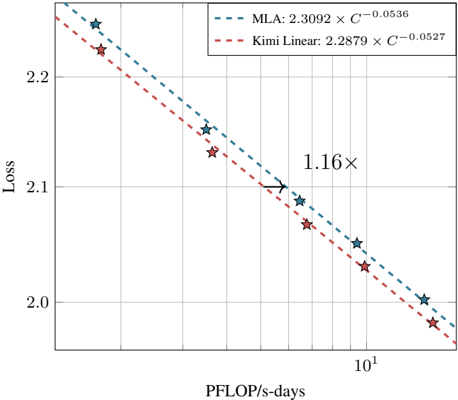
The image is a technical line chart comparing the scaling laws of two models or methods, labeled "MLA" and "Kimi Linear." It plots model "Loss" against computational resources measured in "PFLOP/s-days." Both series show a decreasing, power-law relationship between loss and compute, with Kimi Linear consistently achieving lower loss for a given amount of compute.
### Components/Axes
* **Chart Type:** Line chart with logarithmic x-axis and linear y-axis.
* **X-Axis:**
* **Label:** `PFLOP/s-days`
* **Scale:** Logarithmic (base 10). Major tick mark visible at `10^1` (10). Minor gridlines suggest ticks at 2, 4, 8, 16, etc.
* **Y-Axis:**
* **Label:** `Loss`
* **Scale:** Linear. Major tick marks and gridlines at `2.0`, `2.1`, and `2.2`.
* **Legend:** Positioned in the top-right corner of the plot area.
* **Entry 1:** `MLA: 2.3092 × C^{-0.0536}` (Represented by a teal dashed line with star markers).
* **Entry 2:** `Kimi Linear: 2.2879 × C^{-0.0527}` (Represented by a red dashed line with diamond markers).
* **Annotation:** The text `1.16×` is placed in the center of the chart, between the two lines, indicating a comparative ratio.
* **Data Series:**
1. **MLA:** A teal, dashed line with star-shaped markers.
2. **Kimi Linear:** A red, dashed line with diamond-shaped markers.
### Detailed Analysis
**Data Series & Trends:**
1. **MLA (Teal, Stars):**
* **Trend:** The line slopes downward from left to right, indicating that Loss decreases as PFLOP/s-days increase.
* **Fitted Equation:** `Loss = 2.3092 × C^{-0.0536}`, where C is compute (PFLOP/s-days).
* **Approximate Data Points (Visual Estimation):**
* At ~2 PFLOP/s-days: Loss ≈ 2.25
* At ~4 PFLOP/s-days: Loss ≈ 2.15
* At ~8 PFLOP/s-days: Loss ≈ 2.08
* At ~16 PFLOP/s-days: Loss ≈ 2.00
2. **Kimi Linear (Red, Diamonds):**
* **Trend:** Also slopes downward, parallel to but consistently below the MLA line.
* **Fitted Equation:** `Loss = 2.2879 × C^{-0.0527}`.
* **Approximate Data Points (Visual Estimation):**
* At ~2 PFLOP/s-days: Loss ≈ 2.22
* At ~4 PFLOP/s-days: Loss ≈ 2.13
* At ~8 PFLOP/s-days: Loss ≈ 2.06
* At ~16 PFLOP/s-days: Loss ≈ 1.98
**Annotation Analysis:**
The `1.16×` annotation is placed between the two lines. Given the context of scaling laws, this most likely indicates that to achieve the same loss value, the MLA method requires approximately 1.16 times more compute (PFLOP/s-days) than the Kimi Linear method. This is a measure of relative computational efficiency.
### Key Observations
1. **Consistent Hierarchy:** The Kimi Linear line is positioned below the MLA line across the entire visible range, demonstrating superior performance (lower loss) for any given compute budget.
2. **Similar Scaling Exponents:** The exponents in the power-law equations are very close (`-0.0536` for MLA vs. `-0.0527` for Kimi Linear). This indicates that both models' loss decreases at a nearly identical *rate* as compute increases. The primary difference is in the scaling coefficient (2.3092 vs. 2.2879).
3. **Log-Linear Relationship:** The straight lines on this semi-log plot (log x, linear y) confirm the power-law relationship between Loss and Compute (C), as described by the equations `Loss ∝ C^{-k}`.
4. **Data Sparsity:** The chart displays only four data points per series, which are used to fit the continuous trend lines.
### Interpretation
This chart is a classic representation of **neural scaling laws**, which model how a model's performance (here, loss) improves predictably with increased computational resources.
* **What the Data Suggests:** The data demonstrates that the "Kimi Linear" method is more **compute-efficient** than "MLA." For the same computational investment (PFLOP/s-days), Kimi Linear yields a lower loss. The `1.16×` factor quantifies this advantage: Kimi Linear achieves a given loss level with roughly 16% less compute than MLA.
* **Relationship Between Elements:** The two lines represent competing or alternative methodologies. Their parallel nature suggests they belong to the same family of scaling behavior but with different base efficiencies. The chart allows for direct comparison of their performance-compute trade-offs.
* **Notable Implications:** The near-identical scaling exponents are significant. They imply that the fundamental "return on investment" for additional compute is similar for both methods. The performance gap is therefore established by the constant coefficient and is likely to persist (in absolute loss terms) as compute scales up, rather than one method eventually overtaking the other. This makes the initial efficiency advantage of Kimi Linear particularly valuable for large-scale training.