## Scatter Plot: Model Performance vs. Computational Resources
### Overview
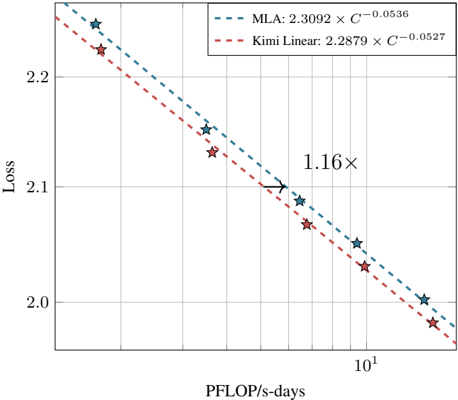
The image is a scatter plot comparing the loss of two models (MLA and Kimi Linear) against computational resources measured in PFLOP/s-days. The plot includes two trend lines (dashed) and annotated data points with stars. A key annotation ("1.16×") highlights a specific data point.
---
### Components/Axes
- **Y-Axis (Loss)**:
- Label: "Loss"
- Scale: Linear, ranging from 2.0 to 2.2 in increments of 0.1.
- Ticks: 2.0, 2.1, 2.2.
- **X-Axis (PFLOP/s-days)**:
- Label: "PFLOP/s-days"
- Scale: Logarithmic, ranging from 10¹ to 10².
- Ticks: 10¹, 10².
- **Legend**:
- Position: Top-right corner.
- Entries:
- **MLA**: Dashed blue line with equation `2.3092 × 10⁻⁰·⁰⁵³⁶`.
- **Kimi Linear**: Dashed red line with equation `2.2879 × 10⁻⁰·⁰⁵²⁷`.
- **Data Points**:
- Symbol: Stars (★).
- Colors: Blue (MLA) and red (Kimi Linear) stars, with some overlapping the trend lines.
---
### Detailed Analysis
- **Trend Lines**:
- **MLA (Blue Dashed Line)**:
- Slope: Slightly decreasing as PFLOP/s-days increase.
- Equation: `Loss = 2.3092 × 10⁻⁰·⁰⁵³⁶`.
- **Kimi Linear (Red Dashed Line)**:
- Slope: Slightly decreasing, parallel to MLA but with a marginally lower loss.
- Equation: `Loss = 2.2879 × 10⁻⁰·⁰⁵²⁷`.
- **Data Points**:
- Stars are distributed along both trend lines, with some points above/below the lines.
- A star at ~10¹ PFLOP/s-days is annotated with "1.16×", pointing to a loss value near 2.1.
---
### Key Observations
1. **Loss vs. Computational Resources**:
- Both models show a **negative correlation** between loss and PFLOP/s-days, indicating improved performance with increased computational resources.
- Kimi Linear consistently achieves **lower loss** than MLA for equivalent PFLOP/s-days.
2. **Annotation "1.16×"**:
- Highlights a data point where the loss is 1.16 times a reference value (context unclear without additional data).
3. **Slope Differences**:
- MLA’s slope (`-0.0536`) is slightly steeper than Kimi Linear’s (`-0.0527`), suggesting MLA’s loss decreases more rapidly with increased resources.
---
### Interpretation
- **Model Efficiency**: Kimi Linear outperforms MLA in terms of loss reduction per unit of computational resource, making it more efficient for the same workload.
- **Trade-offs**: The slight difference in slopes implies MLA may require marginally more resources to achieve similar loss reductions compared to Kimi Linear.
- **Annotation Significance**: The "1.16×" annotation likely emphasizes a critical threshold or benchmark, though its exact meaning depends on the reference value (e.g., baseline loss or target metric).
---
### Spatial Grounding & Verification
- **Legend**: Top-right, clearly associating colors with models.
- **Data Points**: Blue stars align with MLA’s trend line; red stars with Kimi Linear’s. The "1.16×" annotation is spatially linked to a red star near 10¹ PFLOP/s-days.
- **Trend Verification**: Both lines slope downward, confirming the inverse relationship between loss and computational resources.
---
### Content Details
- **Equations**:
- MLA: `2.3092 × 10⁻⁰·⁰⁵³⁶` (≈ 2.3092 × 0.945 ≈ 2.18).
- Kimi Linear: `2.2879 × 10⁻⁰·⁰⁵²⁷` (≈ 2.2879 × 0.946 ≈ 2.16).
- **Loss Values**: All data points fall between 2.0 and 2.2, with Kimi Linear’s values consistently lower.
---
### Final Notes
The plot demonstrates a clear trade-off between computational efficiency and model performance. Kimi Linear’s lower loss and slightly less steep slope suggest it is optimized for resource efficiency, while MLA’s steeper slope indicates faster loss reduction at higher resource levels. The "1.16×" annotation warrants further context to determine its relevance to the analysis.