## Microfluidic Device and Particle Dynamics ### Overview The image presents a two-part illustration of a microfluidic device and the dynamics of a particle within it. Part (a) shows a top-down view of the microfluidic structure, including concentric circular channels and coordinate axes. Part (b) provides a 3D schematic of the device, illustrating the magnetic field, rotation, and a cross-sectional view of a particle trapped in a channel. ### Components/Axes **Part (a): Microfluidic Structure (Top View)** * **Concentric Circular Channels:** The image shows several concentric circular channels etched into a substrate. * **Coordinate Axes:** A coordinate system is superimposed on the image, with the x and y axes intersecting at the center of the circles. * **Angle Φ:** An angle Φ is marked between the x-axis and a radial line. * **Arrows:** A red arrow indicates rotation around the y-axis, and a blue arrow indicates rotation around the center of the circular channels. * **Scale Bar:** A black scale bar is present at the bottom-right of the image. **Part (b): 3D Schematic and Cross-Section** * **3D Schematic:** A 3D representation of the microfluidic device shows a circular channel on a rotating platform. * **Magnetic Field (H):** A blue arrow labeled "H" represents the magnetic field direction. * **Rotation (Ω and ω):** A red arrow labeled "Ω" indicates the rotation of the magnetic field around the z-axis, and a red arrow labeled "ω" indicates the rotation of the platform. * **Coordinate Axes:** A coordinate system is shown, with x, y, and z axes. * **Angle Φ:** An angle Φ is marked between the x-axis and a radial line. * **Cross-Section:** An inset shows a cross-sectional view of the channel with a particle inside. * **Vertical Axis:** Labeled "h[µm]", ranging from -4 to 0. * **Horizontal Axis:** Labeled "ρ[µm]", ranging from 3.5 to 6.5. * **Channel Profile:** A blue line shows the depth profile of the channel. * **Particle:** A pink sphere represents the particle trapped within the channel. ### Detailed Analysis **Part (a): Microfluidic Structure (Top View)** * The concentric circular channels appear to be etched into a flat substrate. * The red arrow indicates a rotation around the y-axis. * The blue arrow indicates a rotation around the center of the circular channels. **Part (b): 3D Schematic and Cross-Section** * The magnetic field (H) is oriented at an angle to the z-axis. * The platform rotates with an angular velocity ω. * The cross-sectional plot shows the depth (h) of the channel as a function of radial position (ρ). * The channel depth is approximately -4 µm. * The channel width is approximately 6.5 µm - 3.5 µm = 3 µm. * The particle is centered within the channel. ### Key Observations * The microfluidic device is designed to trap and manipulate particles using a combination of magnetic fields and rotation. * The cross-sectional plot provides information about the channel geometry and particle position. ### Interpretation The image illustrates a system for manipulating microparticles within a microfluidic device. The combination of a rotating platform and a magnetic field allows for precise control over the particle's motion. The cross-sectional plot provides a detailed view of the channel geometry and the particle's confinement within the channel. This type of system could be used for a variety of applications, including drug delivery, diagnostics, and materials science. The angles and rotations are critical to understanding the forces acting on the particle. The depth profile of the channel is also important for understanding the particle's confinement.

\n ## Diagram: Microfluidic Vortex and Particle Trapping ### Overview The image presents two panels (a and b) illustrating a microfluidic vortex generated within a circular chamber and the trapping of a particle within it. Panel (a) shows a top-down view of the vortex flow pattern, while panel (b) provides a 3D representation of the vortex and a cross-sectional profile of the chamber's height. ### Components/Axes **Panel a:** * **Coordinate System:** A Cartesian coordinate system is overlaid on the image with the x and y axes labeled. An additional radial coordinate, Φ (phi), is also indicated. * **Flow Visualization:** Red and blue arrows depict the direction of fluid flow, forming a vortex pattern. * **Scale Bar:** A black scale bar is present in the bottom-left corner, indicating a length scale (though the exact length is not specified). **Panel b:** * **Coordinate System:** A Cartesian coordinate system (x, y) and a z-axis are shown. * **Vortex Representation:** A gray, conical shape represents the vortex. * **Magnetic Field:** A blue arrow labeled "H" indicates the direction of a magnetic field. * **Rotation Vectors:** A red arrow labeled "Ω" represents the angular velocity of the vortex, and another red arrow labeled "ω" indicates the rotation of the trapped particle. * **Height Profile:** A graph is embedded in the bottom-left corner, plotting height (h) in micrometers (µm) against radial distance (ρ) in micrometers (µm). The axes are labeled "h [µm]" and "ρ [µm]". ### Detailed Analysis or Content Details **Panel a:** The vortex flow pattern is clearly visible as concentric rings. The red arrows indicate a clockwise rotation near the outer edge of the vortex, while the blue arrows indicate a counter-clockwise rotation closer to the center. The flow appears to converge towards the center of the circular chamber. **Panel b:** * **Height Profile:** The embedded graph shows a cross-section of the chamber's height. The height is approximately 0 µm at ρ = 3.5 µm and dips to approximately -4 µm at ρ = 6.5 µm, indicating a concave shape at the bottom of the chamber. The profile shows a rapid increase in height around ρ = 6.5 µm. * **Vortex Orientation:** The vortex is oriented with its apex pointing upwards along the z-axis. * **Magnetic Field and Rotation:** The magnetic field (H) is aligned with the z-axis. The angular velocity of the vortex (Ω) and the particle (ω) are both oriented in the same direction. ### Key Observations * The vortex is generated within a circular microfluidic chamber. * A particle is trapped near the center of the vortex. * The chamber has a non-flat bottom, as evidenced by the height profile. * A magnetic field is present and may be involved in the particle trapping mechanism. ### Interpretation The diagram illustrates a microfluidic system designed to trap particles using a vortex flow. The vortex is likely generated by applying a tangential force to the fluid within the chamber. The particle is drawn into the center of the vortex and held there by the balancing forces of the fluid flow and potentially a magnetic field. The concave shape of the chamber bottom, as shown in the height profile, may contribute to the stability of the vortex and the particle trapping. The magnetic field (H) could be used to manipulate the particle's position or orientation within the vortex. The coordinate systems provide a framework for quantifying the flow dynamics and particle behavior. The diagram suggests a potential application in microfluidic particle sorting, concentration, or analysis.

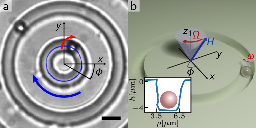
\n ## Diagram: Microscale Rotational System ### Overview The image consists of two panels, labeled **a** and **b**, which together illustrate a physical system involving a particle in a circular micro-trap. Panel **a** is a top-down microscopy image showing concentric circular patterns and overlaid coordinate axes and motion indicators. Panel **b** is a 3D schematic diagram explaining the system's geometry, forces, and a cross-sectional profile of the trapping potential. ### Components/Axes **Panel a (Microscopy Image):** * **Image Type:** Grayscale microscopy image (likely optical or electron). * **Overlaid Graphics:** * **Coordinate System:** A standard Cartesian coordinate system with axes labeled **x** (horizontal, pointing right) and **y** (vertical, pointing up). The origin is at the center of the concentric circles. * **Angle:** An angle **φ** (phi) is marked between the positive x-axis and a radial line extending into the fourth quadrant. * **Motion Indicators:** * A **red curved arrow** near the top of the inner circles indicates a clockwise rotation around the y-axis. * A **blue curved arrow** on the left side indicates a larger, counter-clockwise circular path or flow. * **Scale Bar:** A solid black horizontal bar is present in the bottom-right corner. **No numerical scale value is provided.** **Panel b (3D Schematic):** * **Main Diagram:** * **Central Structure:** A translucent, light-blue cylinder or post. * **Coordinate System:** A 3D Cartesian system with axes labeled **x**, **y**, and **z** (vertical). * **Vectors and Parameters:** * **H:** A blue arrow representing a magnetic field vector, pointing diagonally up and to the right from the cylinder's top. * **Ω (Omega):** A red curved arrow around the z-axis at the top of the cylinder, indicating an angular velocity or rotation of the field/structure. * **φ (phi):** The same angle as in panel **a**, shown between the x-axis and the projection of the **H** vector onto the xy-plane. * **ω (omega):** A red curved arrow around a spherical particle, indicating its orbital angular velocity. The particle is shown on a circular track or groove. * **Inset Graph (Bottom-Left of Panel b):** * **Type:** A 2D line plot showing a cross-sectional profile. * **Y-axis:** Labeled **h [µm]** (height in micrometers). Ticks are at **0** and **-4**. * **X-axis:** Labeled **ρ [µm]** (radial distance in micrometers). Ticks are at **3.5** and **6.5**. * **Data:** A blue line forms a U-shaped or well-shaped profile. A pink/red sphere is depicted sitting at the bottom of this well, centered between ρ = 3.5 µm and ρ = 6.5 µm. ### Detailed Analysis * **Panel a - Spatial Grounding:** The concentric circles suggest a fabricated micro-structure, like a circular channel or potential well. The red arrow (rotation) is positioned over the innermost bright ring. The blue arrow (orbit) is positioned over a darker, outer ring. The coordinate origin is precisely at the center of the pattern. * **Panel b - Component Isolation:** * **Header/Top:** Defines the driving forces: a rotating magnetic field (**H** with angular velocity **Ω**) applied to the system. * **Main Region:** Shows the physical layout: a central post, a circular track around it, and a spherical particle on that track. The particle's motion (**ω**) is coupled to the field's rotation. * **Footer/Inset:** Provides quantitative data on the trap geometry. The graph shows the particle is confined in a radial potential well. The well's bottom is at a height of approximately **h = -4 µm**. The particle's equilibrium position is at a radial distance **ρ ≈ 5.0 µm** (midpoint between 3.5 and 6.5 µm). The well width at the top (h=0) is approximately **3.0 µm** (from 3.5 to 6.5 µm). ### Key Observations 1. **Dual Representation:** The figure pairs an experimental observation (a) with a theoretical/model schematic (b) of the same phenomenon. 2. **Coordinate Consistency:** The angle **φ** and the x-y coordinate system are consistently defined in both panels, linking the experimental image to the model. 3. **Color-Coded Physics:** In panel **b**, **red** is used for angular velocities (**Ω**, **ω**), and **blue** is used for the magnetic field vector (**H**) and the potential well profile, creating a visual association between related concepts. 4. **Scale Discrepancy:** Panel **a** has a scale bar but no value. Panel **b**'s inset provides explicit micrometer-scale dimensions, suggesting the structures in **a** are on the order of 10s of micrometers in diameter. ### Interpretation This figure describes a **magnetically driven microrobotic or microfluidic system**. The data suggests the following mechanism: A spherical particle is trapped in a circular micro-groove (as quantified by the potential well in the inset of **b**). An external, rotating magnetic field (**H** with angular velocity **Ω**) is applied. This field exerts a torque on the particle (likely if it is magnetic or paramagnetic), causing it to orbit the central post with angular velocity **ω**. Panel **a** provides experimental evidence of such circular motion (blue arrow) within the fabricated concentric structure. The red arrow in **a** may indicate the direction of the driving field's rotation. The system demonstrates controlled, non-contact manipulation of a micro-particle using dynamic magnetic fields, with applications in micro-robotics, lab-on-a-chip devices, or studying active matter. The precise alignment of coordinates (**φ**) between experiment and model is crucial for quantitative analysis and control.

## Diagram: Rotational Dynamics and Magnetic Field Interaction ### Overview The image consists of two parts: - **a**: A circular interference pattern with labeled axes (x, y) and angular displacement (φ). Red and blue arrows indicate rotational directions. - **b**: A 3D schematic of a conical structure with vectors (Ω, H, ω) and an inset graph showing height (h) vs. radial distance (ρ). ### Components/Axes #### Part a: - **Axes**: - x-axis (horizontal) and y-axis (vertical) labeled with standard Cartesian coordinates. - Angular displacement φ (phi) marked near the origin. - **Arrows**: - Red arrow: Clockwise rotation (↔). - Blue arrow: Counter-clockwise rotation (↔). - **Scale bar**: 10 µm (bottom-right corner). #### Part b: - **3D Diagram**: - Conical structure with apex labeled Ω (angular velocity, red vector). - Blue vector H (magnetic field) intersecting the cone. - Gray vector ω (angular displacement) on the right. - **Inset Graph**: - Axes: - Radial distance ρ (µm) on the x-axis (3.5–6.5 µm). - Height h (µm) on the y-axis (-4 to 0 µm). - Blue line: Represents a measured profile with a dip at ρ ≈ 5 µm. - **Legend**: - Red: Ω (angular velocity). - Blue: H (magnetic field). - Gray: ω (angular displacement). ### Detailed Analysis #### Part a: - The circular pattern suggests wave interference or rotational motion. - Red and blue arrows indicate opposing rotational directions (clockwise vs. counter-clockwise). - φ (angular displacement) is centered at the origin, with axes x and y defining the plane. #### Part b: - **3D Diagram**: - Ω (red) points upward along the z-axis, indicating rotational motion. - H (blue) is perpendicular to Ω, suggesting a magnetic field aligned with the y-axis. - ω (gray) represents angular displacement, oriented tangentially. - **Inset Graph**: - The blue line shows a parabolic trend with a minimum at ρ ≈ 5 µm (h ≈ -3 µm). - Scale bar: 10 µm (bottom-right corner). ### Key Observations 1. **Part a**: - Opposing rotational directions (red vs. blue arrows) may represent competing forces or wave polarizations. - The scale bar (10 µm) provides spatial context for the interference pattern. 2. **Part b**: - The inset graph’s dip at ρ ≈ 5 µm suggests a localized minimum in height, possibly due to resonance or field interaction. - The 3D vectors (Ω, H, ω) imply a relationship between rotational motion, magnetic fields, and angular displacement. ### Interpretation - **Part a**: The interference pattern and rotational arrows likely model a system with competing rotational dynamics, such as vortices or polarized waves. - **Part b**: The 3D diagram and inset graph suggest a physical system where angular velocity (Ω) and magnetic fields (H) interact to produce a measurable height profile (h) as a function of radial distance (ρ). The dip at ρ ≈ 5 µm could indicate a critical interaction point (e.g., magnetic trapping or resonance). - **Cross-Referencing**: The legend in part b confirms color coding for vectors, ensuring alignment with the 3D model and inset graph. ### Uncertainties - Approximate values (e.g., ρ ≈ 5 µm, h ≈ -3 µm) are inferred from the inset graph’s scale and trend. - The exact nature of the rotational motion (e.g., fluid dynamics vs. electromagnetic) is not explicitly stated.