\n
## Line Chart: Accuracy vs. Lambda with Inset Plot
### Overview
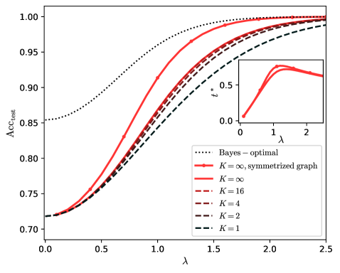
The image displays a technical line chart plotting estimated accuracy (`Acc_est`) against a parameter lambda (`λ`). It includes multiple data series representing different model configurations and a theoretical optimum. A smaller inset plot is embedded within the main chart area, showing the relationship between a different variable (`ℓ*`) and `λ`.
### Components/Axes
**Main Chart:**
* **X-axis:** Label is `λ` (lambda). Scale ranges from 0.0 to 2.5, with major ticks at 0.0, 0.5, 1.0, 1.5, 2.0, 2.5.
* **Y-axis:** Label is `Acc_est` (estimated accuracy). Scale ranges from 0.70 to 1.00, with major ticks at 0.70, 0.75, 0.80, 0.85, 0.90, 0.95, 1.00.
* **Legend:** Located in the bottom-right quadrant of the main chart. It contains seven entries, each with a line style/color sample and a label:
1. `Bayes-optimal` (black, dotted line)
2. `K = ∞, symmetrized graph` (red, solid line)
3. `K = ∞` (red, dashed line)
4. `K = 16` (red, dash-dot line)
5. `K = 4` (black, dashed line)
6. `K = 2` (black, dash-dot line)
7. `K = 1` (black, long-dash line)
**Inset Plot (Top-Right Quadrant):**
* **X-axis:** Label is `λ`. Scale ranges from 0 to 2, with major ticks at 0, 1, 2.
* **Y-axis:** Label is `ℓ*` (ell-star). Scale ranges from 0.0 to approximately 0.8, with major ticks at 0.0, 0.5.
* **Data Series:** A single red, solid line (matching the style for `K = ∞, symmetrized graph` from the main legend).
### Detailed Analysis
**Main Chart Trends & Data Points:**
All curves show a monotonically increasing trend of `Acc_est` as `λ` increases, with diminishing returns as they approach an asymptote near 1.0.
1. **Bayes-optimal (Black Dotted):**
* **Trend:** Starts highest and maintains the highest accuracy across the entire range, approaching 1.0 most rapidly.
* **Approximate Points:** (λ=0.0, Acc≈0.85), (λ=0.5, Acc≈0.90), (λ=1.0, Acc≈0.96), (λ=1.5, Acc≈0.99), (λ=2.0, Acc≈1.00).
2. **K = ∞, symmetrized graph (Red Solid):**
* **Trend:** Starts at the lowest point among all series but rises steeply, converging towards the Bayes-optimal line. It is the highest of the non-optimal curves for λ > ~0.3.
* **Approximate Points:** (λ=0.0, Acc≈0.72), (λ=0.5, Acc≈0.80), (λ=1.0, Acc≈0.92), (λ=1.5, Acc≈0.98), (λ=2.0, Acc≈0.995).
3. **K = ∞ (Red Dashed):**
* **Trend:** Follows a very similar path to the symmetrized version but is consistently slightly lower.
* **Approximate Points:** (λ=0.0, Acc≈0.72), (λ=0.5, Acc≈0.79), (λ=1.0, Acc≈0.91), (λ=1.5, Acc≈0.97), (λ=2.0, Acc≈0.99).
4. **K = 16 (Red Dash-Dot):**
* **Trend:** Rises more slowly than the K=∞ curves. It is the lowest of the red lines.
* **Approximate Points:** (λ=0.0, Acc≈0.72), (λ=0.5, Acc≈0.78), (λ=1.0, Acc≈0.89), (λ=1.5, Acc≈0.96), (λ=2.0, Acc≈0.98).
5. **K = 4 (Black Dashed):**
* **Trend:** Rises more slowly than the K=16 curve.
* **Approximate Points:** (λ=0.0, Acc≈0.72), (λ=0.5, Acc≈0.77), (λ=1.0, Acc≈0.87), (λ=1.5, Acc≈0.94), (λ=2.0, Acc≈0.97).
6. **K = 2 (Black Dash-Dot):**
* **Trend:** Rises more slowly than the K=4 curve.
* **Approximate Points:** (λ=0.0, Acc≈0.72), (λ=0.5, Acc≈0.76), (λ=1.0, Acc≈0.85), (λ=1.5, Acc≈0.92), (λ=2.0, Acc≈0.96).
7. **K = 1 (Black Long-Dash):**
* **Trend:** The slowest rising curve, remaining the lowest for all λ > 0.
* **Approximate Points:** (λ=0.0, Acc≈0.72), (λ=0.5, Acc≈0.75), (λ=1.0, Acc≈0.83), (λ=1.5, Acc≈0.90), (λ=2.0, Acc≈0.94).
**Inset Plot Analysis:**
* **Trend:** The single red curve (corresponding to `K = ∞, symmetrized graph`) shows `ℓ*` increasing sharply from near 0 at λ=0 to a peak, then gradually decreasing.
* **Approximate Key Points:** The peak occurs at approximately λ ≈ 1.3, where `ℓ*` ≈ 0.75. The value at λ=2.0 is approximately `ℓ*` ≈ 0.65.
### Key Observations
1. **Hierarchy of Performance:** There is a clear performance hierarchy: Bayes-optimal > K=∞ (symmetrized) > K=∞ > K=16 > K=4 > K=2 > K=1. This order is maintained across the entire λ range shown.
2. **Convergence:** All non-optimal curves converge towards the Bayes-optimal performance as λ increases, suggesting that a larger λ compensates for model limitations (lower K).
3. **Starting Point:** All non-optimal curves (K=1 through K=∞) originate from the same approximate accuracy (~0.72) at λ=0, while the Bayes-optimal starts significantly higher (~0.85).
4. **Inset Peak:** The inset reveals a non-monotonic relationship for `ℓ*` with respect to λ for the symmetrized K=∞ model, indicating an optimal λ value (~1.3) that maximizes this particular metric.
### Interpretation
This chart likely illustrates the performance of a statistical learning or estimation algorithm (e.g., community detection, clustering) where `K` represents a model complexity parameter (like the number of communities or clusters) and `λ` is a signal-to-noise ratio or regularization parameter.
* **Core Message:** Increasing the signal strength (`λ`) improves estimation accuracy (`Acc_est`) for all model complexities. However, models with higher complexity (`K=∞`) can achieve near-optimal (Bayes-optimal) performance if the signal is strong enough, while simpler models (`K=1,2`) require a much stronger signal to approach the same accuracy.
* **Trade-off Illustrated:** The inset plot for `ℓ*` (which could represent a learned parameter like community size or a loss function) shows that for the most complex model (`K=∞, symmetrized`), there is an intermediate `λ` that maximizes this internal metric. This suggests a potential trade-off or phase transition in the model's behavior as the signal strength varies.
* **Symmetrization Benefit:** The `K=∞, symmetrized graph` curve consistently outperforms the standard `K=∞` curve, indicating that symmetrizing the input graph (a common preprocessing step) provides a tangible accuracy benefit across all signal levels.
* **Practical Implication:** The chart demonstrates that model selection (`K`) is less critical in high-signal regimes (large λ), as all models perform well. In low-signal regimes (small λ), using a more complex model (higher K) is essential to achieve reasonable accuracy. The Bayes-optimal line serves as a theoretical upper bound, showing the fundamental limit of estimation given the data.