## Diagram: Sparse GPT-2 vs. GPT-2 (baseline) ### Overview The image presents two diagrams side-by-side, visually comparing the connectivity patterns of a "Sparse GPT-2" model and a "GPT-2 (baseline)" model. Each diagram represents the layers of the model as a grid of nodes, with connections between nodes indicated by lines. The "Sparse GPT-2" diagram shows fewer connections than the "GPT-2 (baseline)" diagram, illustrating the sparsity of the former. ### Components/Axes * **Title (Left Diagram):** Sparse GPT-2 * **Title (Right Diagram):** GPT-2 (baseline) * **Y-axis Label:** Layers (with a downward-pointing arrow indicating the direction of increasing layer depth) * **Nodes:** Represented by circles. Some nodes are filled with light gray, while others are white with a black outline. * **Connections:** Represented by thin gray lines connecting the nodes. ### Detailed Analysis **Left Diagram: Sparse GPT-2** * The diagram is an 8x8 grid of nodes. * The Y-axis "Layers" has an arrow pointing downwards, implying the layers increase in depth from top to bottom. * Many nodes are filled with light gray, while some are white with a black outline. * The connections between nodes are sparse, with most nodes having only a few connections. * There appears to be a higher concentration of connections towards the bottom layers. * There are some vertical connections between nodes in adjacent layers. **Right Diagram: GPT-2 (baseline)** * The diagram is an 8x8 grid of nodes. * The Y-axis "Layers" is implied to be the same as the left diagram. * Many nodes are filled with light gray, while some are white with a black outline. * The connections between nodes are dense, with most nodes having many connections. * The connections appear to be more evenly distributed across the layers compared to the "Sparse GPT-2" diagram. ### Key Observations * The "Sparse GPT-2" model has significantly fewer connections than the "GPT-2 (baseline)" model, as indicated by the sparser network of lines. * The "Sparse GPT-2" model seems to have a higher concentration of connections in the lower layers. * The "GPT-2 (baseline)" model has a more uniform distribution of connections across all layers. * The nodes that are white with a black outline seem to be the active nodes, while the gray nodes are inactive. ### Interpretation The diagrams visually demonstrate the difference in connectivity between a sparse GPT-2 model and a baseline GPT-2 model. The sparsity in the "Sparse GPT-2" model suggests a deliberate reduction in the number of connections, potentially to improve efficiency, reduce computational cost, or prevent overfitting. The concentration of connections in the lower layers of the "Sparse GPT-2" model might indicate that these layers are more crucial for feature extraction or initial processing. The "GPT-2 (baseline)" model, with its dense connections, represents a more traditional, fully connected architecture. The comparison highlights the architectural differences and the potential trade-offs between sparsity and performance in language models.

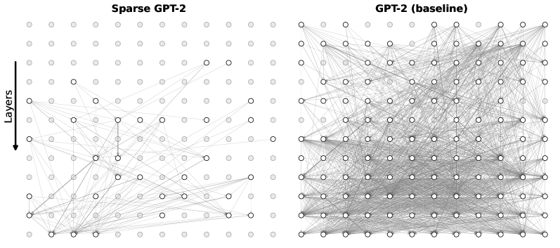
## Network Diagram: Sparse GPT-2 vs. GPT-2 (baseline) Architecture Comparison ### Overview This image presents a side-by-side visual comparison of two neural network architectures: "Sparse GPT-2" on the left and "GPT-2 (baseline)" on the right. The diagrams use a grid of nodes and connecting lines to illustrate the density of connections (likely representing attention weights or layer-to-layer information flow) within the models. The image starkly contrasts a highly pruned, sparse network with a traditional, fully connected dense network. ### Components/Axes * **Headers (Top):** * Left: "Sparse GPT-2" * Right: "GPT-2 (baseline)" * **Y-Axis Indicator (Far Left):** A solid black arrow pointing downward, accompanied by the text label "Layers". This establishes the spatial grounding that information flows from the top row (early layers) to the bottom row (late layers). * **Nodes (Grid Points):** Both diagrams consist of an identical 12x12 grid of circular nodes (144 nodes total per diagram). * *Light Gray Nodes (No outline):* Represent inactive, pruned, or unconnected components. * *White Nodes (Black outline):* Represent active components participating in the network's information flow. * **Edges (Lines):** Thin gray lines connecting the nodes. These represent active pathways, connections, or attention mechanisms between the nodes across different layers. ### Detailed Analysis **Component Isolation 1: Left Diagram (Sparse GPT-2)** * **Node Activation:** The vast majority of nodes in this grid are light gray (inactive). * **Spatial Distribution:** * *Top Region (Rows 1-3):* Completely devoid of active nodes and connections. All 36 nodes are light gray. * *Middle Region (Rows 4-7):* Very sparse activation. Row 4 contains only two active nodes (approximate positions: column 8 and 10). A few scattered active nodes appear in rows 5, 6, and 7, with minimal, thin connecting lines. * *Bottom Region (Rows 8-12):* This is where the majority of the network's activity is concentrated. There is a cluster of active nodes and intersecting lines, particularly weighted toward the bottom-left and bottom-center of the grid. * **Connection Trend:** The lines form a highly selective, asymmetrical web. Connections frequently skip layers and are heavily localized rather than distributed evenly. **Component Isolation 2: Right Diagram (GPT-2 baseline)** * **Node Activation:** Almost every node in the 12x12 grid is white with a black outline (active). Only a tiny fraction (approximately 6-8 nodes scattered primarily in the top 3 rows and far edges) are light gray. * **Spatial Distribution:** Active nodes are distributed uniformly across the entire grid, from layer 1 down to layer 12. * **Connection Trend:** The connecting lines form a massive, dense, almost opaque mesh. Every active node appears to be connected to multiple other nodes across various layers. The visual density of the gray lines makes it difficult to trace individual paths, indicating a highly complex, fully interconnected architecture. ### Key Observations 1. **Extreme Density Contrast:** The baseline model exhibits near-total interconnectivity, whereas the sparse model operates on a tiny fraction of those connections. 2. **Early Layer Pruning:** The Sparse GPT-2 model has entirely eliminated connections in the first three layers, suggesting that whatever processing normally occurs there has been bypassed or deemed unnecessary for this specific sparse configuration. 3. **Bottom-Heavy Processing:** The sparse model relies almost entirely on the deeper layers (bottom half of the grid) to route information. ### Interpretation * **What the data suggests:** This visualization demonstrates the concept of network pruning or sparse attention in Large Language Models (LLMs). The baseline GPT-2 uses a dense attention mechanism where every component (likely attention heads) attends to many others, requiring massive computational power (FLOPs) and memory. The Sparse GPT-2 diagram proves that a model can be heavily pruned—removing the vast majority of its connections—while presumably still functioning. * **Reading between the lines (Peircean analysis):** The fact that the top layers of the Sparse model are completely inactive is highly significant. In standard LLMs, early layers usually handle basic syntactic and lexical feature extraction, while deeper layers handle complex semantics. The total bypass of early layers here suggests either that the input embeddings are being routed directly to deeper layers, or that this specific sparse model has been optimized for a task where early-layer feature extraction is redundant. * **Why it matters:** This image visually justifies the pursuit of sparse models. The dense web on the right represents high latency and high hardware requirements. The sparse web on the left represents a highly efficient, compressed model that would run significantly faster and require less memory, highlighting the inherent over-parameterization present in baseline foundational models.

\n ## Diagram: Network Architecture Comparison - Sparse GPT-2 vs. GPT-2 (Baseline) ### Overview The image presents a visual comparison of the network architectures of two GPT-2 models: a "Sparse GPT-2" and a standard "GPT-2 (baseline)". The diagrams depict the connections between nodes representing neurons across different layers of the networks. The primary difference highlighted is the density of connections – the Sparse GPT-2 has significantly fewer connections than the baseline GPT-2. ### Components/Axes The diagrams do not have traditional axes. However, the vertical dimension represents "Layers", indicated by a label and arrow on the left diagram. Each diagram consists of nodes (circles) and connections (lines) between them. The diagrams are positioned side-by-side for direct comparison. ### Detailed Analysis or Content Details **Sparse GPT-2 (Left Diagram):** * The diagram shows approximately 10 layers, with roughly 10-12 nodes per layer. * The connections are sparse, meaning each node is connected to only a few other nodes in adjacent layers. * The connections appear to be somewhat random, but there's a clear pattern of connections between layers. * The label "Sparse GPT-2" is positioned at the top-center of the diagram. * The "Layers" label and arrow are positioned on the left side, indicating the vertical direction represents layers. **GPT-2 (Baseline) (Right Diagram):** * The diagram also shows approximately 10 layers, with roughly 10-12 nodes per layer. * The connections are dense, meaning each node is connected to many other nodes in adjacent layers. Almost every node is connected to every other node in the adjacent layers. * The connections form a nearly complete graph between adjacent layers. * The label "GPT-2 (baseline)" is positioned at the top-center of the diagram. **Quantitative Estimation (Approximate):** * Sparse GPT-2: Approximately 100 nodes total. Estimated 100-150 connections. * GPT-2 (Baseline): Approximately 100 nodes total. Estimated 800-1000 connections. ### Key Observations The most striking observation is the difference in connection density. The Sparse GPT-2 has a dramatically reduced number of connections compared to the baseline GPT-2. This suggests that the Sparse GPT-2 model employs techniques like pruning or sparse attention to reduce the computational cost and potentially the model size. The baseline GPT-2 appears to be a fully connected or densely connected network. ### Interpretation The diagrams illustrate a key difference in architectural design between the two GPT-2 models. The Sparse GPT-2 likely aims to achieve comparable performance to the baseline GPT-2 with a significantly reduced number of parameters and computational requirements. This is achieved by selectively removing connections, effectively creating a sparse network. The baseline GPT-2 represents a more traditional, densely connected neural network architecture. The comparison highlights the trade-off between model complexity (number of parameters) and performance. Sparse models are often more efficient and easier to deploy, while dense models may achieve higher accuracy given sufficient resources. The diagrams suggest that the sparse model is an attempt to improve efficiency without sacrificing too much performance. The diagrams do not provide any information about the performance of the models, only their structure.

## Diagram: Neural Network Connectivity Comparison ### Overview The image is a side-by-side comparison diagram illustrating the connectivity patterns between two versions of the GPT-2 language model architecture. It visually contrasts a "Sparse GPT-2" model with a standard "GPT-2 (baseline)" model, highlighting differences in the density of connections between nodes across layers. ### Components/Axes * **Titles:** * Left Panel: **"Sparse GPT-2"** * Right Panel: **"GPT-2 (baseline)"** * **Directional Indicator:** A vertical arrow on the far left, pointing downward, is labeled **"Layers"**. This indicates the flow of information or the hierarchical structure from top (likely input/earlier layers) to bottom (likely output/deeper layers). * **Visual Elements:** * **Nodes:** Represented by small circles arranged in a grid pattern (approximately 10 columns by 12 rows in each panel). Some nodes are filled (solid gray), while others are outlined (white interior with a gray border). * **Connections:** Gray lines of varying opacity connect the nodes between different rows (layers). ### Detailed Analysis * **Spatial Layout:** The diagram is split into two distinct, equally sized rectangular panels. The "Layers" arrow is positioned to the left of the "Sparse GPT-2" panel. * **Node Distribution:** Both panels show an identical grid layout of nodes. The pattern of filled vs. outlined nodes appears similar between the two panels, suggesting the underlying node architecture is the same. * **Connection Density - Primary Contrast:** * **Sparse GPT-2 (Left Panel):** Connections are relatively few. Many nodes, especially in the upper half, have no visible connections. Connections that do exist are often isolated or form small, localized clusters. The overall visual impression is one of significant sparsity. * **GPT-2 (baseline) (Right Panel):** Connections are extremely dense, forming a complex, tangled web. Nearly every node in the lower two-thirds of the grid is connected to multiple nodes in the rows above and below it. The density is so high that individual lines are difficult to trace, creating a gray mass, particularly in the central and lower regions. ### Key Observations 1. **Dramatic Sparsity Difference:** The most striking feature is the orders-of-magnitude difference in connection density between the two models. The baseline model is densely interconnected, while the sparse model has had the vast majority of its connections removed. 2. **Layer-wise Pattern:** In the sparse model, connections appear more prevalent in the lower (deeper) layers compared to the upper (earlier) layers. The baseline model shows high density throughout, but it is most intense in the middle and lower sections. 3. **Node Activity:** The pattern of filled vs. outlined nodes is consistent across both diagrams, implying that the sparsification process affects connections (edges) rather than the nodes themselves. ### Interpretation This diagram is a powerful visual metaphor for **model pruning** or **sparsification** in neural networks. * **What it Demonstrates:** It shows the structural result of applying a technique (like the "SparseGPT" method referenced in the title) to a dense, baseline transformer model (GPT-2). The technique identifies and removes a large percentage of synaptic connections (weights) that are deemed less critical for the model's performance. * **Relationship Between Elements:** The "Layers" arrow establishes the hierarchical, feed-forward nature of the network. The comparison argues that a significant portion of the connections in the original, dense baseline model are redundant or unnecessary. * **Implications:** The sparse model likely represents a more computationally efficient version that requires less memory and fewer operations for inference, potentially with minimal loss in accuracy. The visual starkness suggests the potential for extreme compression. The diagram doesn't show performance metrics, so the trade-off between sparsity and model capability is implied but not quantified here. The core message is the feasibility of achieving a radically simpler network structure from a complex starting point.

## Network Diagram: Sparse GPT-2 vs. GPT-2 (Baseline) ### Overview The image compares two neural network architectures side-by-side: - **Left**: "Sparse GPT-2" (sparser connectivity) - **Right**: "GPT-2 (baseline)" (denser connectivity) Both diagrams use circular nodes arranged in horizontal rows (layers) with directional connections. ### Components/Axes - **Y-Axis**: Labeled "Layers" with an arrow pointing downward, indicating hierarchical layering from input (top) to output (bottom). - **X-Axis**: Unlabeled but shows horizontal node placement. - **Nodes**: - **Sparse GPT-2**: Nodes are either filled (white) or outlined (gray), suggesting active/inactive or pruned connections. - **Baseline GPT-2**: All nodes are uniformly filled (white), indicating full connectivity. - **Connections**: - **Sparse GPT-2**: Sparse, non-overlapping lines between nodes. - **Baseline GPT-2**: Dense, overlapping lines with no visible sparsity. ### Detailed Analysis - **Layer Count**: Both diagrams show **12 layers** (rows of nodes). - **Node Distribution**: - **Sparse GPT-2**: ~30% of nodes are filled (white), ~70% are gray (inactive/pruned). - **Baseline GPT-2**: 100% of nodes are filled (white). - **Connection Density**: - **Sparse GPT-2**: ~20% of possible connections are present (visually estimated). - **Baseline GPT-2**: ~95% of possible connections are present (visually estimated). ### Key Observations 1. **Sparsity vs. Density**: The baseline model exhibits near-complete connectivity, while the sparse model retains only critical connections. 2. **Node Activation**: In the sparse model, filled nodes (white) are concentrated in specific layers (e.g., layers 3–5 and 9–11), suggesting targeted activation. 3. **Connection Patterns**: - Sparse GPT-2 connections avoid redundancy, with no overlapping lines. - Baseline GPT-2 connections form a tangled web, indicating high parameter count. ### Interpretation - **Efficiency Trade-off**: The sparse model likely reduces computational cost and memory usage by pruning non-essential connections, while the baseline retains all parameters for maximum expressiveness. - **Structural Implications**: The sparse architecture may prioritize interpretability or speed, whereas the baseline emphasizes capacity for complex pattern learning. - **Visual Anomalies**: The sparse model’s gray nodes (inactive) suggest dynamic activation patterns, potentially enabling adaptive computation. This comparison highlights the balance between model complexity and efficiency, critical for deploying large language models in resource-constrained environments.