## 3D Surface Plot: Unlabeled Mathematical Function
### Overview
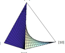
The image displays a three-dimensional surface plot rendered with a wireframe grid and a color gradient. The plot visualizes a mathematical function over a defined domain, showing a surface that curves dramatically from a high point on one side down to a low plane on the other. No chart title is present.
### Components/Axes
* **Axes Labels & Markers:**
* **X-axis:** The axis extends horizontally. At the far right end, the label `[10]` is present. Near the origin (bottom-left corner of the plot area), the number `10` is visible.
* **Y-axis:** The axis extends vertically. At the top end, the label `[10]` is present.
* **Z-axis (Vertical):** The axis extends vertically. At the top-left peak of the plotted surface, the label `[10]` is present.
* **Legend:** There is no separate legend. The color of the surface itself acts as a visual indicator of the Z-axis value (height).
* **Spatial Grounding:** The plot is viewed from an isometric perspective. The origin (0,0,0) appears to be at the bottom-left corner where the axes meet. The `[10]` labels indicate the maximum values on each axis, suggesting the plotted domain is likely from 0 to 10 for X and Y, and the Z-value also ranges up to 10.
### Detailed Analysis
* **Surface Shape & Trend:** The surface exhibits a strong, non-linear trend. It starts at a high point (Z ≈ 10) along the left edge (where X is low and Y is high). As X increases (moving right) and Y decreases (moving down), the surface curves sharply downward, flattening out as it approaches the bottom-right corner (where X is high and Y is low, Z ≈ 0). The shape resembles a hyperbolic paraboloid or a similar saddle-like function, but with one dominant curved slope.
* **Color Gradient:** The surface uses a color gradient to encode height (Z-value). The highest points (top-left) are a deep, dark blue. The color transitions through shades of blue to a light cyan or pale blue at the lowest points (bottom-right). This provides a clear visual cue for the function's value.
* **Grid Overlay:** A wireframe grid is superimposed on the surface. The grid lines follow the contours of the function, becoming more densely packed in areas of steep curvature (the central slope) and more spread out on the flatter regions. This helps in perceiving the 3D shape and the rate of change.
### Key Observations
1. **Monotonic Decrease:** The function appears to be monotonically decreasing along the diagonal from the (X=0, Y=10) corner to the (X=10, Y=0) corner.
2. **Steep Central Slope:** The most dramatic change in Z occurs along the central diagonal of the XY plane, where the surface drops rapidly.
3. **Asymptotic Behavior:** The surface seems to approach the Z=0 plane asymptotically as X approaches 10 and Y approaches 0, rather than intersecting it sharply.
4. **Symmetry:** The plot suggests a potential symmetry or inverse relationship between the X and Y variables in determining the Z value.
### Interpretation
This plot likely represents a function of two variables, `z = f(x, y)`, where the output `z` decreases as the product or some combined measure of `x` and `y` increases. Common functions with this shape include `z = 1/(x*y)` or `z = 10 - sqrt(x^2 + y^2)` within the first quadrant, though the exact formula cannot be determined without explicit labels.
The visualization effectively communicates a strong inverse relationship. In a practical context, this could model phenomena like:
* The decay of a signal or force with distance from a source in two dimensions.
* A utility or production function with diminishing returns.
* A probability density function concentrated near one axis.
The absence of a title, specific axis labels (beyond the max value `[10]`), and a legend limits precise interpretation. The key takeaway is the clear, visual demonstration of a smooth, continuous, and sharply decreasing bivariate relationship. The grid and color gradient are essential for understanding the topology of the function's output space.