## Scatter Plot with Density Contours: Dimensionality Reduction Visualization
### Overview
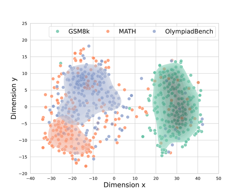
This image is a 2D scatter plot visualizing the distribution of data points across two dimensions, labeled "Dimension x" and "Dimension y". Three distinct categories of data points are represented by different colors: "GSM8k" (teal), "MATH" (orange), and "OlympiadBench" (blue). Density contours are overlaid for each category, indicating regions of higher data point concentration.
### Components/Axes
* **X-axis**: Labeled "Dimension x". The scale ranges approximately from -40 to 50. Major tick marks are present at intervals of 10.
* **Y-axis**: Labeled "Dimension y". The scale ranges approximately from -20 to 25. Major tick marks are present at intervals of 5.
* **Legend**: Located in the top-center of the plot. It associates colors with data categories:
* Teal dots represent "GSM8k".
* Orange dots represent "MATH".
* Blue dots represent "OlympiadBench".
* **Data Points**: Individual points plotted according to their x and y coordinates.
* **Density Contours**: Shaded regions representing the density of points for each category. The contours are semi-transparent, allowing the underlying points to be visible.
### Detailed Analysis or Content Details
**Data Series Trends and Distributions:**
* **GSM8k (Teal):**
* **Trend:** The teal data points are primarily clustered in a dense region on the right side of the plot, roughly between x-coordinates 20 and 40, and y-coordinates 0 and 15. There are a few scattered points outside this main cluster, including one at approximately x=25, y=15, and another at x=25, y=-15.
* **Approximate Extents:** The main cluster spans roughly x=[20, 40] and y=[0, 15]. The density contour for GSM8k is a roughly oval shape centered around x=30, y=7.
* **MATH (Orange):**
* **Trend:** The orange data points are distributed in two main areas. One significant cluster is located in the bottom-left quadrant, roughly between x-coordinates -35 and -15, and y-coordinates -15 and -2. Another, smaller cluster is interspersed with the blue and teal points in the central and right-central regions of the plot.
* **Approximate Extents:** The main bottom-left cluster spans roughly x=[-35, -15] and y=[-15, -2]. The density contour for MATH in this region is an elongated oval shape centered around x=-25, y=-8. Scattered orange points are also observed around x=[0, 30] and y=[-5, 15].
* **OlympiadBench (Blue):**
* **Trend:** The blue data points form a large, diffuse cluster in the central-left to central region of the plot, roughly between x-coordinates -30 and 10, and y-coordinates -5 and 18. There are also some blue points scattered throughout the other regions, particularly mixed with the teal points on the right.
* **Approximate Extents:** The main blue cluster spans roughly x=[-30, 10] and y=[-5, 18]. The density contour for OlympiadBench is a large, irregular shape centered around x=-10, y=6.
**Specific Data Points (Illustrative Examples):**
* **GSM8k:**
* A point at approximately (28, 8) is within the densest part of the teal cluster.
* A point at approximately (35, 12) is also within the main teal cluster.
* A point at approximately (25, -15) is an outlier from the main teal cluster.
* **MATH:**
* A point at approximately (-25, -10) is within the densest part of the bottom-left orange cluster.
* A point at approximately (-30, -5) is also within this cluster.
* A point at approximately (25, 5) is an orange point located within the main teal cluster.
* **OlympiadBench:**
* A point at approximately (-10, 5) is within the densest part of the blue cluster.
* A point at approximately (0, 15) is also within this cluster.
* A point at approximately (30, 10) is a blue point located within the main teal cluster.
### Key Observations
* **Distinct Clustering:** The three categories exhibit distinct clustering patterns, suggesting they represent different types of data or entities that can be separated in this reduced dimensional space.
* **Separation of MATH:** The "MATH" category appears to be the most separated, with a prominent cluster in the bottom-left quadrant that is largely distinct from the other two categories.
* **Overlap and Intermingling:** While there are distinct clusters, there is also significant overlap and intermingling, particularly between "GSM8k" and "OlympiadBench" in the right-central region, and to a lesser extent, "MATH" points are found within the "OlympiadBench" cluster.
* **Outliers:** Each category has some points that lie far from their main cluster, indicating potential anomalies or data points that are less representative of their group.
### Interpretation
This visualization likely represents the output of a dimensionality reduction technique (such as t-SNE or UMAP) applied to datasets from "GSM8k", "MATH", and "OlympiadBench". The plot suggests that these datasets, when projected into a 2D space, form distinct groups.
* **Data Separation:** The clear separation of the "MATH" cluster indicates that this dataset has unique characteristics that distinguish it from "GSM8k" and "OlympiadBench" in the learned latent space.
* **Relationship between GSM8k and OlympiadBench:** The significant overlap between "GSM8k" and "OlympiadBench" suggests that these two datasets share many common features or are structurally similar in the context of the dimensionality reduction. They might represent related tasks or domains.
* **Potential for Classification/Clustering:** The visual separation and clustering imply that a classifier or clustering algorithm could potentially be trained on this reduced-dimensional data to distinguish between these categories with a reasonable degree of accuracy.
* **Outlier Analysis:** The scattered points outside the main clusters could be indicative of data points that are mislabeled, represent edge cases, or are simply less typical examples of their respective categories. Further investigation into these outliers might reveal interesting insights.
In essence, the plot demonstrates the effectiveness of the dimensionality reduction in revealing underlying structures and relationships within the data, highlighting both the distinctiveness and the similarities between the three categories.