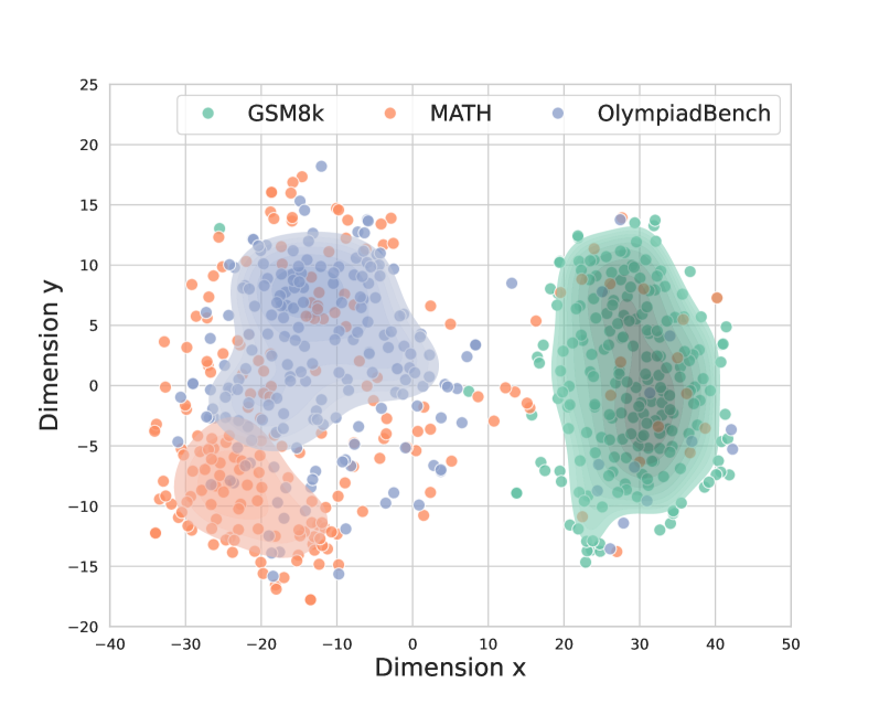
\n ## Scatter Plot: Dimensionality Reduction of Benchmarks ### Overview This image presents a scatter plot visualizing the distribution of three different benchmarks – GSM8k, MATH, and OlympiadBench – across two dimensions (Dimension x and Dimension y). The plot appears to be the result of a dimensionality reduction technique (like PCA or t-SNE) applied to some higher-dimensional data representing these benchmarks. The points are colored to distinguish between the benchmarks, and semi-transparent shading indicates density. ### Components/Axes * **X-axis:** Labeled "Dimension x", ranging from approximately -40 to 50. * **Y-axis:** Labeled "Dimension y", ranging from approximately -20 to 25. * **Legend:** Located in the top-center of the plot. * GSM8k: Represented by teal circles. * MATH: Represented by orange circles. * OlympiadBench: Represented by blue circles. * **Data Points:** Scatter plot points representing individual data instances from each benchmark. * **Shading:** Semi-transparent shading around each cluster of points, indicating density. ### Detailed Analysis The plot shows three distinct clusters of points, corresponding to the three benchmarks. * **GSM8k (Teal):** This cluster is located in the right portion of the plot, centered around Dimension x = 30 and Dimension y = 5. The points are spread out, with a range of Dimension x values from approximately 15 to 45 and Dimension y values from approximately -5 to 15. The density appears highest around (30, 5) and decreases as you move away from this point. * **MATH (Orange):** This cluster is located in the left-center portion of the plot, centered around Dimension x = -20 and Dimension y = -10. The points are relatively tightly clustered, with a range of Dimension x values from approximately -35 to -10 and Dimension y values from approximately -15 to -5. The density is highest around (-20, -10). * **OlympiadBench (Blue):** This cluster is located in the left portion of the plot, centered around Dimension x = -10 and Dimension y = 5. The points are spread out, with a range of Dimension x values from approximately -25 to 10 and Dimension y values from approximately 0 to 15. The density appears highest around (-10, 5) and decreases as you move away from this point. There are a few outliers for each benchmark, points that are distant from the main cluster. For example, there are a few blue points (OlympiadBench) with Dimension x values greater than 20. ### Key Observations * The three benchmarks are clearly separable in this two-dimensional space, suggesting that the dimensionality reduction has successfully captured some underlying differences between them. * MATH appears to be the most tightly clustered benchmark, indicating that its data instances are more similar to each other than those of GSM8k or OlympiadBench. * GSM8k and OlympiadBench have more spread-out distributions, suggesting greater diversity within those benchmarks. * The shading indicates that GSM8k and OlympiadBench have higher densities in certain regions, while MATH has a more uniform density within its cluster. ### Interpretation This plot likely represents a visualization of embeddings generated from a language model or a similar system applied to the three benchmarks. The fact that the benchmarks are separable suggests that the model learns different representations for each benchmark. The tightness of the MATH cluster could indicate that the problems in the MATH benchmark are more homogeneous in terms of the skills or knowledge required to solve them. The spread of GSM8k and OlympiadBench could reflect the greater variety of problem types and difficulty levels within those benchmarks. The dimensionality reduction technique used (likely PCA or t-SNE) has reduced the complexity of the original data while preserving the relative distances between data points. This allows for a visual assessment of the relationships between the benchmarks. The outliers could represent unusual or challenging instances within each benchmark. The plot provides a high-level overview of the characteristics of each benchmark and how they differ from each other. It could be used to inform further analysis or to guide the development of more effective models for solving problems in these domains.