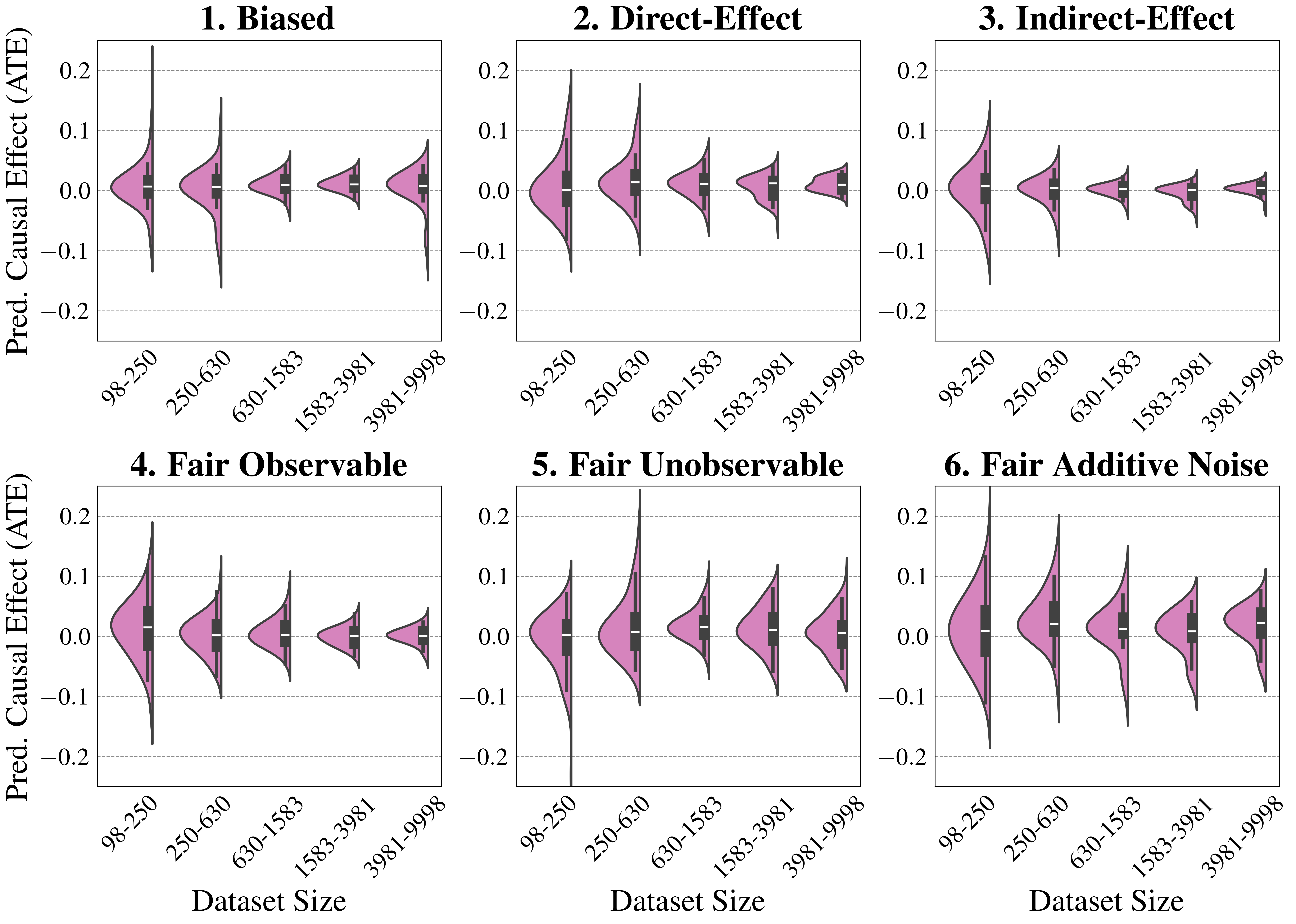
## Violin Plot Grid: Predicted Causal Effect (ATE) by Dataset Size and Method ### Overview The image displays a 2x3 grid of six violin plots. Each subplot visualizes the distribution of the **Predicted Average Treatment Effect (ATE)** for a different causal estimation method across five increasing dataset size categories. The plots compare how the precision and bias of the ATE estimates change with more data for each method. ### Components/Axes * **Overall Layout:** Six subplots arranged in two rows and three columns. * **Subplot Titles (Methods):** 1. **Biased** (Top Left) 2. **Direct-Effect** (Top Center) 3. **Indirect-Effect** (Top Right) 4. **Fair Observable** (Bottom Left) 5. **Fair Unobservable** (Bottom Center) 6. **Fair Additive Noise** (Bottom Right) * **Y-Axis (Common to all subplots):** Labeled **"Pred. Causal Effect (ATE)"**. The scale ranges from -0.2 to 0.2, with major grid lines at intervals of 0.1. * **X-Axis (Common to all subplots):** Labeled **"Dataset Size"**. It contains five categorical bins representing ranges of dataset sizes: * `98-250` * `250-630` * `630-1583` * `1583-3981` * `3981-9998` * **Plot Elements:** Each category on the x-axis has a corresponding **violin plot**. The violin shows the probability density of the data at different values, with a wider section indicating a higher frequency of data points. Inside each violin is a miniature **box plot** (black bar with white median line and whiskers), summarizing the median, interquartile range, and range of the distribution. ### Detailed Analysis The analysis is segmented by subplot (method). For each, the visual trend of the distributions as dataset size increases is described, followed by approximate data points. **1. Biased** * **Trend:** The distributions are centered near zero but show significant spread, especially for smaller datasets. The variance (spread of the violin) decreases noticeably as dataset size increases. The median (white line) remains close to zero across all sizes. * **Data Points (Approximate Median & Spread):** * `98-250`: Median ~0.0, wide spread from ~-0.15 to +0.25. * `250-630`: Median ~0.0, spread narrows (~-0.1 to +0.15). * `630-1583`: Median ~0.0, spread continues to narrow. * `1583-3981`: Median ~0.0, relatively tight distribution. * `3981-9998`: Median ~0.0, tightest distribution, but with a long tail extending to ~-0.15. **2. Direct-Effect** * **Trend:** Similar to "Biased," distributions are centered near zero and variance decreases with more data. The initial spread for the smallest dataset appears slightly larger than in the "Biased" plot. * **Data Points (Approximate Median & Spread):** * `98-250`: Median ~0.0, very wide spread from ~-0.15 to +0.2. * `250-630`: Median ~0.0, spread narrows. * `630-1583`: Median ~0.0, spread narrows further. * `1583-3981`: Median ~0.0, tight distribution. * `3981-9998`: Median ~0.0, very tight distribution. **3. Indirect-Effect** * **Trend:** Distributions are centered near zero. The variance reduction with increasing dataset size is very pronounced. The smallest dataset shows a particularly wide and tall distribution. * **Data Points (Approximate Median & Spread):** * `98-250`: Median ~0.0, extremely wide and tall distribution (high density around zero but large range). * `250-630`: Median ~0.0, spread reduces dramatically. * `630-1583`: Median ~0.0, tight distribution. * `1583-3981`: Median ~0.0, very tight distribution. * `3981-9998`: Median ~0.0, extremely tight distribution. **4. Fair Observable** * **Trend:** Distributions are centered near zero. Variance decreases with dataset size. The shape and spread appear very similar to the "Biased" method. * **Data Points (Approximate Median & Spread):** * `98-250`: Median ~0.0, wide spread. * `250-630`: Median ~0.0, spread narrows. * `630-1583`: Median ~0.0, spread narrows further. * `1583-3981`: Median ~0.0, tight distribution. * `3981-9998`: Median ~0.0, tight distribution. **5. Fair Unobservable** * **Trend:** This method shows a distinct pattern. While the median remains near zero, the **variance does not decrease consistently** with dataset size. The distributions for the two largest dataset sizes (`1583-3981` and `3981-9998`) appear wider than those for the middle sizes, suggesting instability or increased uncertainty with more data for this method. * **Data Points (Approximate Median & Spread):** * `98-250`: Median ~0.0, wide spread. * `250-630`: Median ~0.0, spread narrows. * `630-1583`: Median ~0.0, relatively tight. * `1583-3981`: Median ~0.0, spread increases again. * `3981-9998`: Median ~0.0, spread remains wide. **6. Fair Additive Noise** * **Trend:** Distributions are centered near zero. Variance decreases with dataset size, but the rate of decrease appears slower compared to methods like "Indirect-Effect." The distributions remain relatively wide even for larger datasets. * **Data Points (Approximate Median & Spread):** * `98-250`: Median ~0.0, very wide spread. * `250-630`: Median ~0.0, spread narrows. * `630-1583`: Median ~0.0, spread narrows further. * `1583-3981`: Median ~0.0, moderately wide distribution. * `3981-9998`: Median ~0.0, moderately wide distribution. ### Key Observations 1. **Universal Trend:** For five of the six methods (all except "Fair Unobservable"), the variance (uncertainty) of the predicted ATE decreases as the dataset size increases. This is the expected behavior of consistent estimators. 2. **Bias:** All methods appear to be **unbiased** on average, as the median of every distribution is centered at or very near 0.0 on the y-axis. 3. **Method Comparison:** * The **"Indirect-Effect"** method shows the most dramatic reduction in variance, achieving the tightest distributions for large datasets. * The **"Fair Unobservable"** method is an outlier. Its variance does not monotonically decrease and is notably high for the largest datasets, indicating potential issues with this estimation approach under the tested conditions. * The **"Biased"** and **"Fair Observable"** methods show very similar performance profiles. * The **"Fair Additive Noise"** method retains higher variance than others at large dataset sizes. ### Interpretation This visualization is a comparative performance analysis of different causal inference methods. The **Predicted ATE** is the estimated average effect of a treatment or intervention. The plots reveal how the **precision** (inverse of variance) of these estimates improves with more data. * **What the data suggests:** Most methods become more precise with larger datasets, which validates their statistical consistency. The "Indirect-Effect" method appears most efficient in this test. The anomalous behavior of "Fair Unobservable" suggests that incorporating unobservable confounders in a fairness-aware model may introduce instability or require a different modeling approach that doesn't scale well with data size in this scenario. * **How elements relate:** The x-axis (Dataset Size) is the independent variable. The y-axis (Predicted ATE) is the dependent variable whose distribution is measured. The subplot titles (Methods) are the different models or algorithms being tested. The violin shape directly visualizes the uncertainty in the causal estimate for each method at each data scale. * **Notable anomalies:** The primary anomaly is the **"Fair Unobservable"** method's failure to reduce variance with the largest datasets. This could indicate overfitting, model misspecification, or a fundamental challenge in estimating causal effects when accounting for unobservable factors in a fairness context. The long tail in the largest dataset for the "Biased" method is a minor secondary anomaly.