## Bias vs. Variance Plot for Learning Algorithms ### Overview The image is a 2D scatter plot illustrating the relationship between bias and variance for different learning algorithms. The x-axis represents variance (randomness in weight changes), and the y-axis represents bias (gradient, weight change). Several algorithms are positioned on the plot based on their relative bias and variance. ### Components/Axes * **X-axis:** Variance, i.e., randomness in weight changes. The axis increases from left to right. * **Y-axis:** Bias, i.e., gradient, weight change. The axis increases from bottom to top. * **Data Points:** Represent different learning algorithms. ### Detailed Analysis The following algorithms are plotted: * **Error backpropagation:** Located at the origin (bottom-left corner), indicating low bias and low variance. * **Contrastive learning, predictive coding, dendritic error:** Located on the y-axis, above error backpropagation, indicating low variance and moderate bias. There is a question mark next to this label. * **Feedback alignment:** Located on the y-axis, higher than the previous point, indicating low variance and high bias. * **AGREL:** Located on the x-axis, to the right of the origin, indicating low bias and moderate variance. There is a question mark next to this label. * **Node perturbation:** Located on the x-axis, further to the right than AGREL, indicating low bias and higher variance. * **Weight perturbation:** Located on the x-axis, furthest to the right, indicating low bias and the highest variance among the plotted algorithms. * **RDD:** Located in the upper-right quadrant, indicating moderate bias and moderate variance. There is a question mark next to this label. ### Key Observations * Algorithms on the y-axis (Error backpropagation, Contrastive learning, Feedback alignment) have low variance. * Algorithms on the x-axis (Error backpropagation, AGREL, Node perturbation, Weight perturbation) have low bias. * The plot suggests a trade-off between bias and variance. ### Interpretation The plot visually represents the bias-variance trade-off in machine learning. Algorithms like "Error backpropagation" aim for both low bias and low variance, while others prioritize one over the other. "Feedback alignment" exhibits high bias and low variance, potentially indicating underfitting. "Weight perturbation" exhibits low bias and high variance, potentially indicating overfitting. The question marks next to "Contrastive learning, predictive coding, dendritic error", "AGREL", and "RDD" suggest uncertainty or variability in their exact placement on the bias-variance spectrum. The plot helps in understanding the characteristics of different learning algorithms in terms of their bias and variance properties.

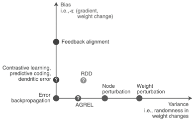
\n ## Scatter Plot: Learning Algorithms and Their Characteristics ### Overview The image presents a scatter plot illustrating the relationship between "Bias" (vertical axis) and "Variance" (horizontal axis) for various learning algorithms. Each algorithm is represented by a point on the plot, and question marks indicate uncertainty or areas requiring further investigation. ### Components/Axes * **X-axis:** Labeled "Variance", with the clarifying text "i.e., randomness in weight changes". The scale is not explicitly marked, but appears to range from low variance on the left to high variance on the right. * **Y-axis:** Labeled "Bias", with the clarifying text "i.e., ∇ (gradient, weight change)". The scale is not explicitly marked, but appears to range from low bias at the bottom to high bias at the top. * **Data Points/Algorithms:** * Feedback alignment * Contrastive learning, predictive coding, dendritic error * RDD (with a question mark) * AGREL (with a question mark) * Node perturbation * Weight perturbation * Error backpropagation * **Question Marks:** Placed near the data points for "RDD" and "AGREL", and also near "Contrastive learning, predictive coding, dendritic error", indicating uncertainty in their precise positioning or characteristics. ### Detailed Analysis The plot shows a general trend of increasing variance as bias decreases. * **Feedback alignment:** Located in the top-left quadrant, indicating high bias and low variance. Approximate coordinates: (1, 9). * **Contrastive learning, predictive coding, dendritic error:** Located in the upper-middle quadrant, indicating high bias and moderate variance. Approximate coordinates: (3, 7). * **Error backpropagation:** Located in the lower-middle quadrant, indicating low bias and moderate variance. Approximate coordinates: (3, 2). * **AGREL:** Located near the x-axis, indicating low bias and low variance. Approximate coordinates: (4, 1). * **RDD:** Located between AGREL and Contrastive learning, predictive coding, dendritic error, indicating low bias and moderate variance. Approximate coordinates: (5, 4). * **Node perturbation:** Located on the x-axis, indicating low bias and high variance. Approximate coordinates: (6, 1). * **Weight perturbation:** Located on the x-axis, indicating low bias and very high variance. Approximate coordinates: (7, 1). The positioning of the algorithms suggests a trade-off between bias and variance. Algorithms with high bias tend to have low variance, and vice versa. ### Key Observations * The algorithms cluster along a diagonal, suggesting a negative correlation between bias and variance. * The question marks highlight areas where the positioning of the algorithms is uncertain or requires further investigation. * Error backpropagation, AGREL, Node perturbation, and Weight perturbation are positioned relatively close to the x-axis, indicating low bias. * Feedback alignment and Contrastive learning, predictive coding, dendritic error are positioned relatively high on the y-axis, indicating high bias. ### Interpretation This plot illustrates a fundamental concept in machine learning: the bias-variance trade-off. Algorithms with high bias make strong assumptions about the data, leading to low variance but potentially high errors if the assumptions are incorrect. Algorithms with low bias make fewer assumptions, leading to high variance and potentially overfitting the data. The positioning of the algorithms on the plot suggests their relative strengths and weaknesses. For example, Feedback alignment is a high-bias, low-variance algorithm, which might be suitable for simple problems where strong assumptions are valid. Weight perturbation is a low-bias, high-variance algorithm, which might be suitable for complex problems where flexibility is important. The question marks indicate that the positioning of RDD, AGREL, and Contrastive learning, predictive coding, dendritic error is uncertain, suggesting that further research is needed to understand their characteristics. The plot provides a useful visual representation of the trade-off between bias and variance, and can help guide the selection of appropriate learning algorithms for different problems.

## Diagram: Conceptual Map of Learning Mechanisms and Perturbations ### Overview The diagram illustrates a conceptual framework mapping relationships between learning mechanisms, perturbations, and their alignment with bias/error backpropagation. It uses labeled points connected by directional arrows to represent theoretical connections. ### Components/Axes - **Vertical Axis**: Labeled "Bias (i.e., gradient, weight change)" with an upward arrow. - **Horizontal Axis**: Labeled "Error backpropagation" with a rightward arrow. - **Key Points**: 1. **Feedback alignment** (top-center) 2. **Contrastive learning, predictive coding, dendritic error** (left-center) 3. **RDD** (question mark, mid-left) 4. **Node perturbation** (mid-right) 5. **Weight perturbation** (far-right) 6. **AGREL** (origin point) 7. **Error backpropagation** (bottom-left) - **Additional Labels**: - "Variance (i.e., randomness in weight changes)" (far-right) - Question marks at **RDD** and **AGREL** indicate uncertainty. ### Detailed Analysis - **Feedback alignment** is positioned at the highest vertical point, suggesting maximal alignment with bias/gradient. - **Contrastive learning, predictive coding, dendritic error** cluster near the origin but slightly elevated, indicating partial alignment with bias. - **RDD** (Reinforcement-Driven Dynamics?) is marked with a question mark, implying unresolved theoretical status. - **Node perturbation** and **Weight perturbation** lie along the horizontal axis, showing progression from error backpropagation to variance in weight changes. - **AGREL** (Adaptive Gradient Regularization?) is at the origin, serving as a reference point for perturbations. ### Key Observations 1. **Directional Flow**: Arrows suggest a progression from error backpropagation (bottom-left) to weight perturbation (far-right), with intermediate steps like node perturbation. 2. **Uncertainty Markers**: Question marks at **RDD** and **AGREL** highlight gaps in understanding or empirical validation. 3. **Bias vs. Perturbation Tradeoff**: Higher vertical positioning correlates with stronger bias alignment, while horizontal progression reflects increasing perturbation complexity. ### Interpretation The diagram conceptualizes a spectrum of learning mechanisms and their relationship to bias/error dynamics. It positions **feedback alignment** as the most bias-aligned method, while **contrastive learning** and **predictive coding** occupy a middle ground. The inclusion of **RDD** and **AGREL** as question-marked nodes suggests these are either emerging concepts or areas requiring further research. The horizontal progression from error backpropagation to weight perturbation implies a theoretical framework where perturbations introduce variance, potentially improving generalization but at the cost of increased randomness in weight updates. The diagram emphasizes the need to balance bias alignment with controlled perturbation to optimize learning outcomes.