## 2D Plot: Symmetrical Hysteresis Loops
### Overview
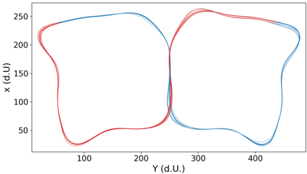
The image displays a 2D Cartesian plot containing two smooth, closed-loop curves. The curves are symmetrical about a vertical axis near the center of the plot. One curve is colored red and is positioned primarily on the left side of the plot. The other curve is colored blue and is positioned primarily on the right side. The plot has labeled axes with numerical scales.
### Components/Axes
* **Vertical Axis (Y-axis):** Labeled `x (d.U.)`. The scale runs from approximately 0 to 250, with major tick marks labeled at 50, 100, 150, 200, and 250.
* **Horizontal Axis (X-axis):** Labeled `Y (d.U.)`. The scale runs from approximately 0 to 450, with major tick marks labeled at 100, 200, 300, and 400.
* **Unit Notation:** Both axes use the unit `(d.U.)`, which likely stands for "digital units" or "device units," indicating the data is from a digital sensor or measurement system.
* **Legend:** There is no explicit legend within the image frame. The two data series are distinguished solely by color (red and blue).
### Detailed Analysis
**Spatial Grounding & Trend Verification:**
1. **Red Curve (Left Loop):**
* **Placement:** Occupies the left half of the plot, primarily between Y=0 and Y=250 on the horizontal axis.
* **Trend:** The curve forms a smooth, continuous loop. Starting from the bottom-left near (Y≈50, x≈25), it slopes upward and to the right, reaching a peak near (Y≈100, x≈250). It then curves downward and to the right, crossing the center vertical axis near (Y≈250, x≈100). It continues downward and to the left, reaching a minimum near (Y≈100, x≈25), before looping back up to the starting point.
* **Key Points (Approximate):**
* Bottom-left minimum: (Y≈50, x≈25)
* Top peak: (Y≈100, x≈250)
* Center crossing: (Y≈250, x≈100)
* Bottom-right minimum: (Y≈100, x≈25)
2. **Blue Curve (Right Loop):**
* **Placement:** Occupies the right half of the plot, primarily between Y=250 and Y=450 on the horizontal axis.
* **Trend:** This curve is a near-perfect mirror image of the red curve across the vertical line at Y≈250. Starting from the bottom-right near (Y≈400, x≈25), it slopes upward and to the left, reaching a peak near (Y≈350, x≈250). It then curves downward and to the left, crossing the center vertical axis near (Y≈250, x≈100). It continues downward and to the right, reaching a minimum near (Y≈350, x≈25), before looping back up to the starting point.
* **Key Points (Approximate):**
* Bottom-right minimum: (Y≈400, x≈25)
* Top peak: (Y≈350, x≈250)
* Center crossing: (Y≈250, x≈100)
* Bottom-left minimum: (Y≈350, x≈25)
**Component Isolation:**
* **Header/Title:** No title is present in the image.
* **Main Chart Area:** Contains the two described loops on a white background with a light gray border.
* **Footer/Axis Labels:** The axis labels and numerical tick marks are clearly printed in black.
### Key Observations
1. **Perfect Symmetry:** The most striking feature is the bilateral symmetry of the two loops around the vertical axis at Y≈250. The red and blue curves are mirror images.
2. **Hysteresis Shape:** Both curves exhibit classic hysteresis loop shapes, indicating a system where the output (x) depends not only on the current input (Y) but also on its history (the direction of change).
3. **Shared Crossing Point:** Both loops intersect at a single common point near the center of the plot (Y≈250, x≈100).
4. **Identical Vertical Range:** Both curves span the same vertical range, from x≈25 to x≈250.
5. **Absence of a Legend:** The lack of a legend means the specific meaning of the red vs. blue curves (e.g., loading vs. unloading, increasing vs. decreasing field, two different samples) must be inferred from external context.
### Interpretation
This plot likely represents the **hysteresis loops of a symmetric system or two opposing states**. Hysteresis is common in magnetic materials (magnetization vs. applied field), ferroelectric materials, mechanical systems with friction, and certain control systems.
* **What the Data Suggests:** The symmetry implies that the process being measured behaves identically but in opposite directions. For example, if this were a magnetic material, the red loop could represent the magnetization cycle when an external magnetic field is swept from negative to positive, and the blue loop could represent the cycle when the field is swept from positive to negative. The shared crossing point at (Y≈250, x≈100) might represent a coercive point or a neutral state.
* **How Elements Relate:** The horizontal axis (`Y (d.U.)`) is the independent variable or driving force (e.g., applied field, stress, voltage). The vertical axis (`x (d.U.)`) is the dependent response (e.g., magnetization, strain, polarization). The loop shape shows that the response lags behind the drive, creating a memory effect.
* **Notable Anomalies:** The primary "anomaly" is the perfect symmetry, which in real-world physical systems is often an idealization. Slight imperfections or asymmetries are common. The clean, smooth curves suggest either simulated/theoretical data or a very well-behaved, idealized experimental system.
* **Peircean Investigation:** The sign here is an **icon** (it resembles the physical phenomenon of hysteresis) and an **index** (it points to a causal relationship where the state of the system depends on its past trajectory). The symmetry is an **index** of a balanced, reversible process under ideal conditions. The lack of a legend is a significant **index** that this image is likely a figure from a technical paper or report where the legend is provided in the accompanying caption or text, not in the graphic itself.