## 3D Surface Plot: Minimised Energy Landscape
### Overview
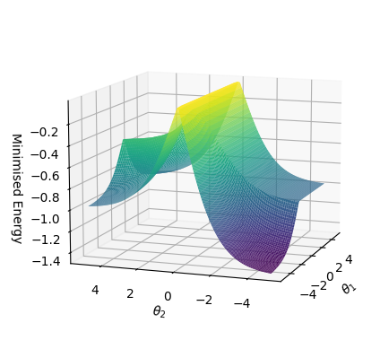
The image depicts a 3D surface plot visualizing a minimised energy landscape as a function of two angular variables, θ₁ and θ₂. The plot uses a color gradient (purple to yellow) to represent energy levels, with a grid overlay for spatial reference. The surface exhibits a central peak and asymmetrical troughs, suggesting a non-uniform energy distribution.
### Components/Axes
- **X-axis (θ₂)**: Ranges from -4 to 4, labeled with increments of 2.
- **Y-axis (θ₁)**: Ranges from -4 to 4, labeled with increments of 2.
- **Z-axis (Minimised Energy)**: Ranges from -1.4 to 0.2, labeled with increments of 0.2.
- **Color Gradient**: Purple (lowest energy) to yellow (highest energy), with no explicit legend but implied by color intensity.
- **Grid**: Black grid lines with spacing consistent across all axes.
### Detailed Analysis
1. **Central Peak**:
- Located at θ₁ ≈ 0, θ₂ ≈ 0.
- Energy value ≈ 0.2 (yellow region).
- Slope: Gradual ascent from surrounding troughs.
2. **Left Trough**:
- Extends from θ₁ ≈ -4 to θ₁ ≈ -2, θ₂ ≈ -4 to 0.
- Energy values ≈ -1.0 to -0.8 (dark blue to green).
- Shape: Bowl-like depression with steep sides.
3. **Right Trough**:
- Extends from θ₁ ≈ 2 to θ₁ ≈ 4, θ₂ ≈ -4 to 0.
- Energy values ≈ -1.2 to -0.6 (purple to blue).
- Shape: Asymmetrical dip with a sharper gradient on the θ₂ > 0 side.
4. **Edge Behavior**:
- Energy values drop to ≈ -1.4 at θ₁ = ±4, θ₂ = ±4 (corners).
- Color transitions from purple (lowest) to green/yellow (highest) across the surface.
### Key Observations
- **Symmetry**: The central peak is symmetric about θ₁ = 0 and θ₂ = 0, but the troughs are asymmetrical.
- **Energy Extremes**:
- Maximum energy: 0.2 (central peak).
- Minimum energy: -1.4 (bottom-right corner).
- **Gradient Steepness**: The right trough has a steeper energy gradient compared to the left trough.
### Interpretation
The plot likely represents a physical or mathematical system where energy minimization depends on angular variables θ₁ and θ₂. The central peak suggests a stable equilibrium at θ₁ = 0, θ₂ = 0, while the troughs indicate metastable states or energy wells. The asymmetry in trough depths and slopes implies external influences or non-linear interactions in the system. The color gradient confirms that energy values are directly proportional to the surface height, with no additional categorical variables. This visualization could be used in fields like physics (e.g., potential energy landscapes) or optimization algorithms to identify global vs. local minima.