## Chart: Minimum Length vs. Time and Tau
### Overview
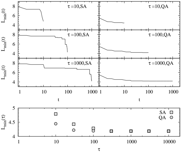
The image presents a series of line graphs and a scatter plot examining the relationship between minimum length (Lmin(t)) and time (t), as well as Lmin(T) and tau (τ). The data is presented for two different methods, labeled "SA" (Simulated Annealing) and "QA" (Quasi-Newton Algorithm). The graphs explore how Lmin(t) changes over time for different values of τ, and how Lmin(T) varies with τ.
### Components/Axes
* **Top Section:** Contains six line graphs arranged in a 3x2 grid.
* **Y-axis (all graphs):** Lmin(t) - labeled "Lmin(t)", ranging from approximately 4 to 8.
* **X-axis (all graphs):** t - labeled "t", on a logarithmic scale from 1 to 1000.
* **Titles (each graph):** Indicate the value of τ and the method used (e.g., "τ=10,SA").
* **Bottom Section:** A scatter plot.
* **Y-axis:** Lmin(T) - labeled "Lmin(T)", ranging from approximately 4 to 5.5.
* **X-axis:** τ - labeled "τ", on a logarithmic scale from 1 to 10000.
* **Legend (top-right):**
* SA (Simulated Annealing) - represented by a black square.
* QA (Quasi-Newton Algorithm) - represented by a white circle.
### Detailed Analysis or Content Details
**Top Section - Line Graphs:**
* **τ=10, SA (Top-Left):** The line starts at approximately 7.8 and rapidly decreases to around 5.5 by t=10. It then plateaus around 5.5 until t=100, after which it decreases slightly to approximately 5.2 by t=1000.
* **τ=10, QA (Top-Right):** The line starts at approximately 7.5 and gradually decreases to around 5.5 by t=1000. The decrease is relatively smooth and consistent.
* **τ=100, SA (Middle-Left):** The line starts at approximately 7.8 and decreases in steps to around 5.2 by t=100. It remains relatively constant until t=1000, where it decreases slightly to approximately 5.0.
* **τ=100, QA (Middle-Right):** The line starts at approximately 7.5 and gradually decreases to around 5.5 by t=1000. The decrease is smoother than the SA method.
* **τ=1000, SA (Bottom-Left):** The line starts at approximately 7.8 and decreases rapidly in steps to around 5.2 by t=100. It remains relatively constant until t=1000, where it decreases slightly to approximately 5.0.
* **τ=1000, QA (Bottom-Right):** The line starts at approximately 7.5 and decreases gradually to around 5.5 by t=1000. The decrease is smoother than the SA method.
**Bottom Section - Scatter Plot:**
* **SA (Black Squares):**
* τ=10: Lmin(T) ≈ 5.3
* τ=100: Lmin(T) ≈ 5.1
* τ=1000: Lmin(T) ≈ 4.9
* τ=10000: Lmin(T) ≈ 4.8
* **QA (White Circles):**
* τ=10: Lmin(T) ≈ 5.1
* τ=100: Lmin(T) ≈ 5.0
* τ=1000: Lmin(T) ≈ 4.9
* τ=10000: Lmin(T) ≈ 4.8
### Key Observations
* For all values of τ, the SA method exhibits a more stepwise decrease in Lmin(t) compared to the smoother decrease observed with the QA method.
* As τ increases, the initial value of Lmin(t) remains relatively constant around 7.8-7.5.
* The final value of Lmin(t) at t=1000 appears to converge towards approximately 5.0-5.5 for both methods and all values of τ.
* The scatter plot shows that Lmin(T) decreases slightly as τ increases for both SA and QA methods. The decrease is more pronounced for the SA method.
* The QA method consistently yields slightly lower values of Lmin(T) compared to the SA method for all values of τ.
### Interpretation
The data suggests that the minimum length (Lmin) decreases over time (t) for both Simulated Annealing (SA) and Quasi-Newton Algorithm (QA) methods. The rate of decrease is influenced by the parameter τ. Larger values of τ seem to lead to a more gradual decrease in Lmin(t) for both methods. The scatter plot indicates that the final minimum length (Lmin(T)) is also affected by τ, with larger τ values resulting in slightly lower Lmin(T).
The difference in the behavior of the two methods (SA vs. QA) is notable. SA exhibits a more discrete, stepwise decrease, likely due to its stochastic nature, while QA demonstrates a smoother, more continuous decrease, characteristic of gradient-based optimization methods. The QA method consistently achieves slightly lower final minimum lengths, suggesting it might be more efficient in finding optimal solutions in this context.
The logarithmic scale on the x-axis (t and τ) indicates that the effects of time and τ are likely non-linear. The initial rapid decrease in Lmin(t) followed by a plateau suggests that the system quickly reaches a state of diminishing returns, where further optimization yields smaller improvements. The convergence of Lmin(t) towards a similar value for all τ values at t=1000 suggests that the system is approaching a stable state, regardless of the initial value of τ.