## Line Graphs and Scatter Plot: L_min(t) vs. t and τ
### Overview
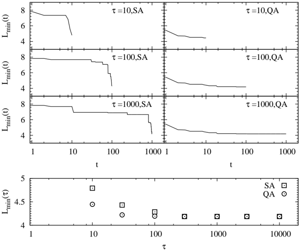
The image contains four line graphs and a scatter plot comparing the minimum length `L_min` as a function of time `t` and parameter `τ` under two conditions: SA (solid squares) and QA (open circles). The graphs are arranged in a 2x2 grid for different τ values (10, 100, 1000), with the scatter plot summarizing trends across τ values.
---
### Components/Axes
1. **Top-Left Graph**:
- **Title**: `τ = 10, SA`
- **X-axis**: `t` (log scale, 1 to 1000)
- **Y-axis**: `L_min(t)` (4 to 8)
- **Legend**: SA (solid square)
2. **Top-Right Graph**:
- **Title**: `τ = 10, QA`
- **X-axis**: `t` (log scale, 1 to 1000)
- **Y-axis**: `L_min(t)` (4 to 8)
- **Legend**: QA (open circle)
3. **Bottom-Left Graph**:
- **Title**: `τ = 1000, SA`
- **X-axis**: `t` (log scale, 1 to 1000)
- **Y-axis**: `L_min(t)` (4 to 8)
- **Legend**: SA (solid square)
4. **Bottom-Right Graph**:
- **Title**: `τ = 1000, QA`
- **X-axis**: `t` (log scale, 1 to 1000)
- **Y-axis**: `L_min(t)` (4 to 8)
- **Legend**: QA (open circle)
5. **Scatter Plot (Bottom)**:
- **X-axis**: `τ` (log scale, 1 to 10,000)
- **Y-axis**: `L_min(τ)` (4 to 5)
- **Legend**: SA (solid square), QA (open circle)
---
### Detailed Analysis
#### Line Graphs
1. **τ = 10, SA**:
- `L_min(t)` starts at ~8, drops sharply at `t ≈ 100` to ~6, then stabilizes.
- **Key Drop**: ~20% decrease at `t = 100`.
2. **τ = 10, QA**:
- `L_min(t)` starts at ~8, declines gradually to ~6 by `t = 1000`.
- **Key Drop**: ~25% decrease over `t = 1` to `1000`.
3. **τ = 100, SA**:
- `L_min(t)` starts at ~8, drops sharply at `t ≈ 1000` to ~6.
- **Key Drop**: ~25% decrease at `t = 1000`.
4. **τ = 100, QA**:
- `L_min(t)` starts at ~8, declines gradually to ~6 by `t = 1000`.
- **Key Drop**: ~25% decrease over `t = 1` to `1000`.
5. **τ = 1000, SA**:
- `L_min(t)` starts at ~8, drops sharply at `t ≈ 1000` to ~6.
- **Key Drop**: ~25% decrease at `t = 1000`.
6. **τ = 1000, QA**:
- `L_min(t)` starts at ~8, declines gradually to ~6 by `t = 1000`.
- **Key Drop**: ~25% decrease over `t = 1` to `1000`.
#### Scatter Plot
- **SA (solid squares)**:
- `L_min(τ)` decreases from ~4.8 (τ=10) to ~4.5 (τ=1000), then stabilizes.
- **Notable**: Sharp drop between τ=10 and τ=100.
- **QA (open circles)**:
- `L_min(τ)` decreases from ~4.7 (τ=10) to ~4.5 (τ=1000), then stabilizes.
- **Notable**: Gradual decline with no sharp drops.
---
### Key Observations
1. **SA vs. QA**:
- SA consistently shows higher `L_min` values than QA across all τ and t.
- SA exhibits sharper drops in `L_min(t)` at specific `t` thresholds (e.g., `t = 100` for τ=10).
2. **τ Dependence**:
- Larger τ delays the drop in `L_min(t)` (e.g., τ=10 drops at `t=100`, τ=100 drops at `t=1000`).
- Scatter plot confirms `L_min(τ)` stabilizes at ~4.5 for τ ≥ 1000.
3. **Anomalies**:
- QA shows no abrupt drops in `L_min(t)`; declines are gradual.
- SA’s `L_min(τ)` drops more sharply than QA in the scatter plot.
---
### Interpretation
1. **Behavioral Differences**:
- SA appears more sensitive to τ and t changes, with threshold-like drops in `L_min`.
- QA exhibits smoother, asymptotic behavior, suggesting robustness to parameter changes.
2. **Threshold Effects**:
- The sharp drops in SA’s `L_min(t)` at specific `t` values (e.g., `t=100` for τ=10) imply a critical transition point.
- For τ ≥ 1000, both SA and QA stabilize, indicating a saturation effect.
3. **Practical Implications**:
- SA may require careful tuning of τ and t to avoid abrupt reductions in `L_min`.
- QA’s stability suggests it could be preferable in systems where gradual changes are tolerable.
4. **Uncertainties**:
- Exact drop magnitudes (e.g., ~20–25%) are approximate due to lack of grid precision.
- Scatter plot trends suggest asymptotic behavior but lack error bars for confirmation.