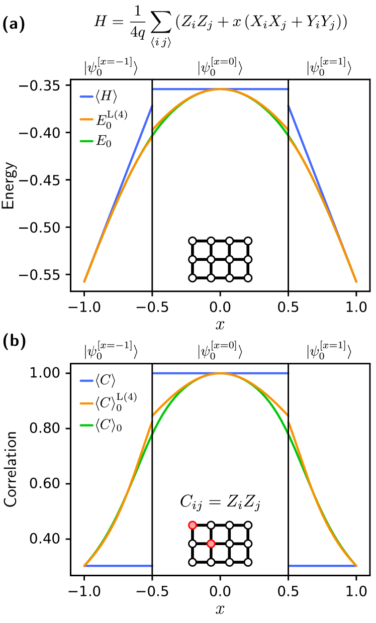
## [Chart/Diagram Type]: Dual-Panel Scientific Plot with Hamiltonian and Correlation Functions ### Overview The image contains two vertically stacked scientific plots, labeled (a) and (b), which analyze the properties of a quantum system on a 2D lattice. Both plots share the same x-axis parameter `x` and are divided into three distinct regions by vertical lines at `x = -0.5` and `x = 0.5`. Each plot compares three different quantities (represented by blue, orange, and green lines) and includes a schematic of a 3x3 square lattice. The overall context appears to be the study of a phase transition or crossover in a quantum many-body system, likely related to the transverse-field Ising model or a similar Hamiltonian. ### Components/Axes **Common Elements:** * **X-axis:** Labeled `x`. Scale ranges from -1.0 to 1.0 with major ticks at -1.0, -0.5, 0.0, 0.5, 1.0. * **Vertical Dividers:** Solid black vertical lines at `x = -0.5` and `x = 0.5`. * **Region Labels (Top of each panel):** Three quantum state notations are placed above the three regions defined by the vertical lines: * Left region (`x < -0.5`): `|ψ₀^{[x=-1]}⟩` * Center region (`-0.5 < x < 0.5`): `|ψ₀^{[x=0]}⟩` * Right region (`x > 0.5`): `|ψ₀^{[x=1]}⟩` * **Lattice Schematic:** A 3x3 grid of circles (sites) connected by lines (bonds) is centered in the lower half of each plot. **Panel (a) Specifics:** * **Title/Label:** `(a)` in the top-left corner. * **Y-axis:** Labeled `Energy`. Scale ranges from -0.55 to -0.35 with major ticks at -0.55, -0.50, -0.45, -0.40, -0.35. * **Legend (Top-Left):** * Blue line: `⟨H⟩` * Orange line: `E₀^{L(4)}` * Green line: `E₀` * **Equation (Top Center):** The Hamiltonian for the system is given as: `H = (1/(4q)) Σ_{<i j>} (Z_i Z_j + x (X_i X_j + Y_i Y_j))` * **Lattice Schematic:** The 3x3 lattice is shown with all sites and bonds in black/white. **Panel (b) Specifics:** * **Title/Label:** `(b)` in the top-left corner. * **Y-axis:** Labeled `Correlation`. Scale ranges from 0.40 to 1.00 with major ticks at 0.40, 0.60, 0.80, 1.00. * **Legend (Top-Left):** * Blue line: `⟨C⟩` * Orange line: `⟨C⟩₀^{L(4)}` * Green line: `⟨C⟩₀` * **Equation (Center):** The correlation function being plotted is defined as: `C_ij = Z_i Z_j` * **Lattice Schematic:** The 3x3 lattice is shown with two specific sites highlighted in red (one at the top-left corner and one at the center of the grid), indicating the pair `(i, j)` for which the correlation `C_ij` is calculated. ### Detailed Analysis **Panel (a) - Energy vs. x:** * **Trend Verification:** * **Blue Line (`⟨H⟩`):** This is a piecewise linear function. It slopes upward from `x = -1.0` to `x = -0.5`, remains constant (flat) at its maximum value from `x = -0.5` to `x = 0.5`, and then slopes downward from `x = 0.5` to `x = 1.0`. * **Orange Line (`E₀^{L(4)}`):** This is a smooth, symmetric, concave-down parabola. It increases from `x = -1.0`, peaks at `x = 0.0`, and then decreases symmetrically to `x = 1.0`. * **Green Line (`E₀`):** This is also a smooth, symmetric, concave-down parabola, very similar in shape to the orange line but consistently slightly lower in energy across the entire range. * **Data Points (Approximate):** * At `x = -1.0`: All three lines converge at approximately `Energy = -0.55`. * At `x = 0.0`: The blue line is at its plateau value of approximately `-0.35`. The orange and green parabolas peak here, with the orange line (`E₀^{L(4)}`) nearly touching the blue line's plateau, and the green line (`E₀`) peaking slightly lower, at approximately `-0.36`. * At `x = 1.0`: All three lines converge again at approximately `Energy = -0.55`. * At the boundaries `x = ±0.5`: The blue line has a sharp corner. The orange and green curves pass through these points smoothly, with values around `-0.40`. **Panel (b) - Correlation vs. x:** * **Trend Verification:** * **Blue Line (`⟨C⟩`):** This is a piecewise constant function with a sharp jump. It is flat at a low value from `x = -1.0` to `x = -0.5`, jumps to a high constant value from `x = -0.5` to `x = 0.5`, and then jumps back down to the low constant value from `x = 0.5` to `x = 1.0`. * **Orange Line (`⟨C⟩₀^{L(4)}`):** This is a smooth, symmetric, concave-down parabola. It increases from `x = -1.0`, peaks at `x = 0.0`, and then decreases symmetrically to `x = 1.0`. * **Green Line (`⟨C⟩₀`):** This is also a smooth, symmetric, concave-down parabola, following the orange line very closely but lying slightly below it across the entire range. * **Data Points (Approximate):** * At `x = -1.0` and `x = 1.0`: The blue line is at its low plateau of approximately `Correlation = 0.30`. The orange and green parabolas start at this same value. * At `x = 0.0`: The blue line is at its high plateau of `Correlation = 1.00`. The orange and green parabolas peak here, with the orange line (`⟨C⟩₀^{L(4)}`) reaching `1.00` and the green line (`⟨C⟩₀`) peaking just below it, at approximately `0.98`. * At the boundaries `x = ±0.5`: The blue line has a vertical jump. The orange and green curves pass through these points smoothly, with values around `0.80`. ### Key Observations 1. **Phase Transition Signatures:** The vertical lines at `x = ±0.5` mark critical points where the behavior of the exact quantities (blue lines) changes abruptly—from sloping to flat in (a), and from low to high in (b). This is characteristic of a first-order phase transition or a sharp crossover. 2. **Approximation Accuracy:** The orange lines (`E₀^{L(4)}` and `⟨C⟩₀^{L(4)}`) appear to be approximations (likely from a 4th-order linked-cluster expansion or similar method) to the exact ground state quantities (green lines: `E₀` and `⟨C⟩₀`). The approximations are excellent, especially near `x=0`, but show slight deviations. 3. **Symmetry:** Both plots are perfectly symmetric about `x = 0.0`, indicating a symmetry in the underlying Hamiltonian (e.g., `x → -x` symmetry). 4. **Correlation Function Behavior:** The correlation `C_ij` for the specific pair highlighted (corner and center sites) is maximal (`1.0`) in the central phase (`|ψ₀^{[x=0]}⟩`) and drops to a constant, lower value (`~0.30`) in the outer phases. This suggests the central phase has strong, possibly long-range, order for this operator. ### Interpretation The data demonstrates the properties of a quantum system governed by the Hamiltonian `H`, which interpolates between different regimes via the parameter `x`. The three regions correspond to distinct quantum phases or ground states, labeled `|ψ₀^{[x=-1]}⟩`, `|ψ₀^{[x=0]}⟩`, and `|ψ₀^{[x=1]}⟩`. * **What the data suggests:** The system undergoes two sharp transitions at `x = ±0.5`. In the outer phases (`|x| > 0.5`), the energy `⟨H⟩` varies linearly with `x`, and the correlation `⟨C⟩` is constant and low. In the central phase (`|x| < 0.5`), the energy is constant (maximized), and the correlation is constant and maximal. This is a classic signature of a system where the ground state changes discontinuously at the critical points. * **Relationship between elements:** The Hamiltonian equation defines the energy being plotted in (a). The correlation function `C_ij = Z_i Z_j` is a specific observable derived from the same Hamiltonian, plotted in (b). The lattice diagrams visually ground the abstract equations, showing the physical system (a 2D square lattice) and, in (b), the specific operator being measured. The state labels at the top identify the ground state wavefunction in each region. * **Notable anomalies/patterns:** The most striking pattern is the "flat-top" behavior of the exact quantities (blue lines) in the central region. This indicates that within this phase, the ground state energy and the specific correlation `⟨C⟩` are *insensitive* to the parameter `x`. This is unusual and points to a highly degenerate or specially symmetric ground state manifold in that phase. The smooth parabolic approximations (orange/green) fail to capture this flatness, highlighting the non-perturbative nature of the transition. The perfect symmetry of the plots confirms the Hamiltonian's symmetry under `x → -x`.