## Chart/Diagram Type: Energy and Correlation Graphs with Lattice Diagrams
### Overview
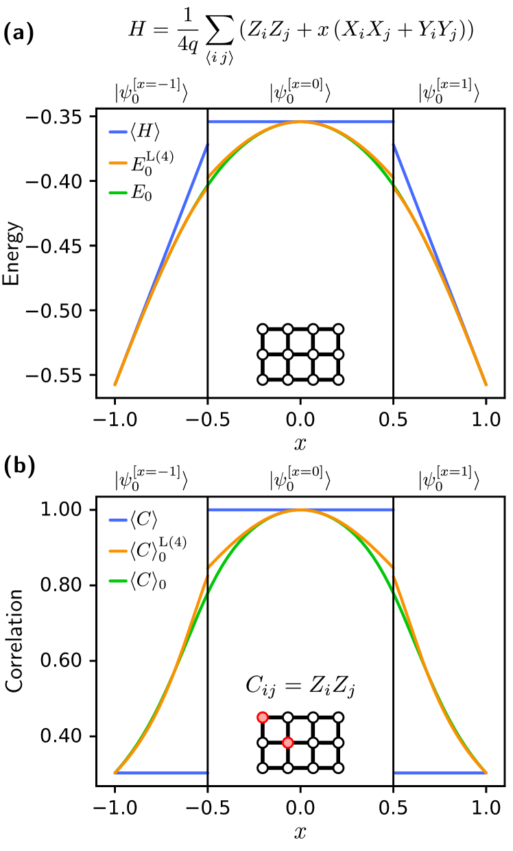
The image contains two panels (a) and (b), each featuring a graph with energy/correlation values plotted against a parameter *x*. Both panels include lattice diagrams below the graphs, with annotations for quantum states and interactions. The graphs compare theoretical predictions (orange) and ground-state values (green) against calculated averages (blue).
---
### Components/Axes
#### Panel (a): Energy Graph
- **Y-axis**: Energy (range: -0.55 to -0.35)
- **X-axis**: Parameter *x* (range: -1.0 to 1.0), divided into three regions:
- |ψ₀^[x=-1]⟩ (left)
- |ψ₀^[x=0]⟩ (center)
- |ψ₀^[x=1]⟩ (right)
- **Legend**:
- Blue: ⟨H⟩ (average Hamiltonian)
- Orange: E₀^L(4) (localized energy)
- Green: E₀ (ground-state energy)
- **Lattice Diagram**: A 3x3 grid of nodes (black circles) with connecting lines.
#### Panel (b): Correlation Graph
- **Y-axis**: Correlation (range: 0.4 to 1.0)
- **X-axis**: Same *x* parameter as panel (a), with identical state labels.
- **Legend**:
- Blue: ⟨C⟩ (average correlation)
- Orange: ⟨C⟩₀^L(4) (localized correlation)
- Green: ⟨C⟩₀ (ground-state correlation)
- **Lattice Diagram**: A 3x3 grid with two red-highlighted nodes connected by a line.
---
### Detailed Analysis
#### Panel (a): Energy Trends
1. **Blue Line (⟨H⟩)**:
- Flat at -0.35 across all *x* values.
- Spatial grounding: Horizontal line spanning the entire x-axis.
2. **Orange Line (E₀^L(4))**:
- Parabolic shape: Peaks at -0.35 (center) and dips to -0.55 at x = ±1.
- Crosses the green line at x ≈ ±0.3.
3. **Green Line (E₀)**:
- Parabolic shape: Peaks at -0.35 (center) and dips to -0.55 at x = ±1.
- Overlaps with orange line at x = 0 but diverges at x = ±1.
#### Panel (b): Correlation Trends
1. **Blue Line (⟨C⟩)**:
- Flat at 1.0 across all *x* values.
- Spatial grounding: Horizontal line at the top of the y-axis.
2. **Orange Line (⟨C⟩₀^L(4))**:
- Parabolic shape: Peaks at 1.0 (center) and dips to 0.4 at x = ±1.
- Crosses the green line at x ≈ ±0.3.
3. **Green Line (⟨C⟩₀)**:
- Parabolic shape: Peaks at 1.0 (center) and dips to 0.4 at x = ±1.
- Overlaps with orange line at x = 0 but diverges at x = ±1.
---
### Key Observations
1. **Symmetry**: Both panels exhibit symmetric behavior around *x* = 0.
2. **State Boundaries**: The vertical dashed lines at x = -1, 0, and 1 demarcate distinct quantum states.
3. **Red Dots in Lattice (Panel b)**: Located at (0,0) and (1,1), suggesting a specific interaction or coupling between these nodes.
4. **Divergence at x = ±1**: Both energy and correlation graphs show sharp drops at the edges of the x-axis, indicating boundary effects.
---
### Interpretation
1. **Hamiltonian and Energy**:
- The flat ⟨H⟩ line (panel a) suggests a constant average energy across all states, while the parabolic E₀^L(4) and E₀ lines indicate localized energy minima at the center state (x = 0).
- The divergence at x = ±1 implies higher energy costs for transitions to these states.
2. **Correlation Function**:
- The flat ⟨C⟩ line (panel b) indicates uniform average correlation, while ⟨C⟩₀^L(4) and ⟨C⟩₀ show maximum correlation at x = 0, decaying symmetrically toward the edges.
- The red-highlighted nodes in the lattice (panel b) likely represent critical coupling points influencing the correlation decay.
3. **Theoretical vs. Ground-State Values**:
- The orange (localized) and green (ground-state) lines in both panels converge at x = 0 but diverge at the edges, suggesting that localized approximations (orange) overestimate energy/correlation compared to ground-state values (green) at x = ±1.
4. **Lattice Dynamics**:
- The 3x3 grid diagrams visually map the system’s spatial structure. The red dots in panel (b) may denote entangled or strongly interacting nodes, critical for understanding the correlation decay.
---
### Conclusion
The graphs illustrate how energy and correlation properties of a quantum system evolve with the parameter *x*, transitioning between distinct states. The lattice diagrams provide spatial context, highlighting key interactions that govern the system’s behavior. The divergence at x = ±1 underscores the sensitivity of the system to boundary conditions, while the central peaks (x = 0) reflect stable, highly correlated states.