## Partition Diagram: Partition of Input Space ### Overview The image is a diagram showing the partition of an input space. The space is divided into rectangular regions by vertical and horizontal lines. The x-axis represents π/3 < x1 < 2π/3, and the y-axis represents π/3 < x2 < 2π/3. The diagram shows how the input space is divided into different regions. ### Components/Axes * **Title:** Partition of input space * **X-axis:** π/3 < x1 < 2π/3, with tick marks at 1.1, 1.2, 1.3, 1.4, 1.5, 1.6, 1.7, 1.8, 1.9, and 2.0. * **Y-axis:** π/3 < x2 < 2π/3, with tick marks at 1.1, 1.2, 1.3, 1.4, 1.5, 1.6, 1.7, 1.8, 1.9, and 2.0. * The diagram is composed of blue lines that partition the space. ### Detailed Analysis The input space is partitioned into rectangular regions. The vertical lines are located at approximately x = 1.2, 1.3, 1.4, 1.5, 1.6, 1.8, 1.9, and 2.0. The horizontal lines are located at approximately y = 1.3, 1.6. * **Region 1 (Bottom-Left):** Bounded by x = 1.1 to 1.2, and y = 1.1 to 1.3. * **Region 2:** Bounded by x = 1.2 to 1.3, and y = 1.1 to 1.3. * **Region 3:** Bounded by x = 1.3 to 1.4, and y = 1.1 to 1.3. * **Region 4:** Bounded by x = 1.4 to 1.5, and y = 1.1 to 1.3. * **Region 5:** Bounded by x = 1.5 to 1.6, and y = 1.1 to 1.3. * **Region 6:** Bounded by x = 1.6 to 1.8, and y = 1.1 to 1.3. * **Region 7:** Bounded by x = 1.8 to 1.9, and y = 1.1 to 1.3. * **Region 8:** Bounded by x = 1.9 to 2.0, and y = 1.1 to 1.3. * **Region 9:** Bounded by x = 2.0 to 2.1, and y = 1.1 to 1.3. * **Region 10:** Bounded by x = 1.1 to 1.3, and y = 1.3 to 1.6. * **Region 11:** Bounded by x = 1.3 to 1.6, and y = 1.3 to 1.6. * **Region 12:** Bounded by x = 1.6 to 2.0, and y = 1.3 to 1.6. * **Region 13:** Bounded by x = 2.0 to 2.1, and y = 1.3 to 1.6. * **Region 14:** Bounded by x = 1.1 to 1.3, and y = 1.6 to 1.85. * **Region 15:** Bounded by x = 1.1 to 1.3, and y = 1.85 to 2.05. * **Region 16:** Bounded by x = 1.3 to 1.6, and y = 1.6 to 2.05. * **Region 17:** Bounded by x = 1.6 to 1.8, and y = 1.6 to 2.05. * **Region 18:** Bounded by x = 1.8 to 2.0, and y = 1.6 to 2.05. * **Region 19:** Bounded by x = 2.0 to 2.1, and y = 1.6 to 2.05. ### Key Observations The partitioning is non-uniform. The regions in the bottom-left corner are smaller than the regions in the top-right corner. ### Interpretation The diagram represents a partitioning of the input space defined by π/3 < x1 < 2π/3 and π/3 < x2 < 2π/3. The partitioning is done using vertical and horizontal lines, creating rectangular regions. This type of partitioning is commonly used in machine learning and control systems to divide the input space into different regions, each of which may be associated with a different action or prediction. The non-uniform partitioning suggests that the regions in the bottom-left corner are more important or require finer granularity than the regions in the top-right corner.

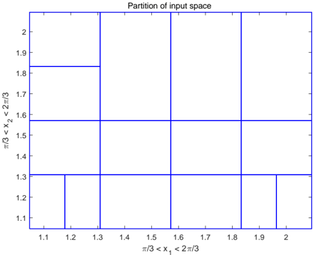
## Diagram: Partition of Input Space ### Overview This image displays a two-dimensional Cartesian plot titled "Partition of input space". It shows a rectangular region divided into multiple smaller, non-uniform rectangular cells by a series of blue horizontal and vertical lines. The axes are labeled with mathematical expressions defining the range of two variables, `x₁` and `x₂`. ### Components/Axes **Title:** * "Partition of input space" (located at the top-center of the plot area). **X-axis (Horizontal Axis):** * **Title:** `π/3 < x₁ < 2π/3` (located below the x-axis, centered). * Numerically, `π/3` is approximately 1.047, and `2π/3` is approximately 2.094. * **Range:** The visible plot area for `x₁` spans from approximately 1.05 to 2.05. * **Tick Markers:** 1.1, 1.2, 1.3, 1.4, 1.5, 1.6, 1.7, 1.8, 1.9, 2.0. **Y-axis (Vertical Axis):** * **Title:** `π/3 < x₂ < 2π/3` (located to the left of the y-axis, rotated vertically). * Numerically, `π/3` is approximately 1.047, and `2π/3` is approximately 2.094. * **Range:** The visible plot area for `x₂` spans from approximately 1.05 to 2.05. * **Tick Markers:** 1.1, 1.2, 1.3, 1.4, 1.5, 1.6, 1.7, 1.8, 1.9, 2.0. **Legend:** * No legend is present in the image. **Plot Area:** * The background of the plot area is white. * The partitioning lines are solid blue. ### Detailed Analysis The plot area represents a 2D input space defined by `x₁` and `x₂`, bounded by the approximate ranges [1.047, 2.094] for both variables. This space is divided into a grid of rectangular cells by a series of blue lines. The partitioning is not uniform. **Horizontal Partitioning Lines (y-coordinates):** The space is primarily divided horizontally by lines at the following y-coordinates, which span the entire width of the plot (from x ≈ 1.047 to x ≈ 2.094): * y = 1.30 * y ≈ 1.57 (between 1.5 and 1.6) * y ≈ 1.83 (between 1.8 and 1.9) **Vertical Partitioning Lines (x-coordinates):** The space is divided vertically by lines at the following x-coordinates: * x ≈ 1.18 (between 1.1 and 1.2): This line only extends from y ≈ 1.047 (bottom boundary) to y = 1.30. * x = 1.30: This line extends across the full height of the plot (from y ≈ 1.047 to y ≈ 2.094). * x ≈ 1.57 (between 1.5 and 1.6): This line extends across the full height of the plot. * x ≈ 1.83 (between 1.8 and 1.9): This line extends across the full height of the plot. * x ≈ 1.95 (between 1.9 and 2.0): This line only extends from y ≈ 1.047 (bottom boundary) to y = 1.30. **Resulting Rectangular Cells:** The combination of these lines creates 18 distinct rectangular regions (cells) within the input space: * **Bottom Row (y from ~1.047 to 1.30):** This row is divided into 6 cells by vertical lines at x ≈ 1.18, x = 1.30, x ≈ 1.57, x ≈ 1.83, and x ≈ 1.95. * Cell 1: x ∈ [~1.047, 1.18], y ∈ [~1.047, 1.30] * Cell 2: x ∈ [1.18, 1.30], y ∈ [~1.047, 1.30] * Cell 3: x ∈ [1.30, 1.57], y ∈ [~1.047, 1.30] * Cell 4: x ∈ [1.57, 1.83], y ∈ [~1.047, 1.30] * Cell 5: x ∈ [1.83, 1.95], y ∈ [~1.047, 1.30] * Cell 6: x ∈ [1.95, ~2.094], y ∈ [~1.047, 1.30] * **Middle Two Rows (y from 1.30 to 1.57, and y from 1.57 to 1.83):** Each of these rows is divided into 4 cells by vertical lines at x = 1.30, x ≈ 1.57, and x ≈ 1.83. * For y ∈ [1.30, 1.57]: * Cell 7: x ∈ [~1.047, 1.30], y ∈ [1.30, 1.57] * Cell 8: x ∈ [1.30, 1.57], y ∈ [1.30, 1.57] * Cell 9: x ∈ [1.57, 1.83], y ∈ [1.30, 1.57] * Cell 10: x ∈ [1.83, ~2.094], y ∈ [1.30, 1.57] * For y ∈ [1.57, 1.83]: * Cell 11: x ∈ [~1.047, 1.30], y ∈ [1.57, 1.83] * Cell 12: x ∈ [1.30, 1.57], y ∈ [1.57, 1.83] * Cell 13: x ∈ [1.57, 1.83], y ∈ [1.57, 1.83] * Cell 14: x ∈ [1.83, ~2.094], y ∈ [1.57, 1.83] * **Top Row (y from 1.83 to ~2.094):** This row is also divided into 4 cells by vertical lines at x = 1.30, x ≈ 1.57, and x ≈ 1.83. * Cell 15: x ∈ [~1.047, 1.30], y ∈ [1.83, ~2.094] * Cell 16: x ∈ [1.30, 1.57], y ∈ [1.83, ~2.094] * Cell 17: x ∈ [1.57, 1.83], y ∈ [1.83, ~2.094] * Cell 18: x ∈ [1.83, ~2.094], y ∈ [1.83, ~2.094] ### Key Observations * The input space is a square region defined by `x₁` and `x₂` both ranging from approximately 1.047 to 2.094. * The partitioning is non-uniform, meaning the resulting rectangular cells have varying widths and heights. * Some vertical partition lines (at x ≈ 1.18 and x ≈ 1.95) do not span the entire height of the plot, indicating a hierarchical or localized refinement of the partition, specifically in the bottom-most region (y from ~1.047 to 1.30). * The major horizontal and vertical partition lines (at x=1.30, x≈1.57, x≈1.83 and y=1.30, y≈1.57, y≈1.83) divide the space into a coarser 4x4 grid, with the bottom-left and bottom-right cells of this coarser grid further subdivided. * The axis labels `π/3` and `2π/3` suggest that the input space might represent angular or phase information, or parameters derived from such quantities. ### Interpretation This diagram illustrates a "partition of input space," which is a common technique in various fields such as numerical analysis, machine learning, control systems, and optimization. The non-uniformity of the cells suggests an adaptive partitioning strategy. Instead of dividing the space into equally sized bins, certain regions (specifically the bottom strip of the `x₂` range, from approximately 1.047 to 1.30) have been further subdivided along the `x₁` axis. This could imply: 1. **Higher Resolution/Sensitivity:** The system or model being analyzed requires finer granularity or more detailed exploration in the region where `x₂` is between ~1.047 and 1.30. This might be an area where the system's behavior is more complex, sensitive to changes in `x₁`, or where critical operating points are located. 2. **Adaptive Sampling/Meshing:** The partition might be the result of an adaptive algorithm that refines the grid based on some criteria, such as error estimates, density of data points, or gradients of a function being optimized. 3. **Feature Importance:** The variables `x₁` and `x₂` are likely input features or parameters. The partitioning indicates that their combined influence on an output or system state is not uniform across the entire domain. The use of `π/3` and `2π/3` in the axis labels strongly hints at applications involving periodic functions, angles, or phase spaces, where these specific values often represent significant points (e.g., 60 degrees and 120 degrees). This type of partitioning could be used for tasks like function approximation, state-space discretization for reinforcement learning, or defining regions for different control strategies. The diagram effectively communicates a structured, yet adaptively refined, decomposition of a 2D parameter domain.

## 2D Plot: Partition of Input Space ### Overview The image displays a 2D Cartesian coordinate plot showing a rectangular area that has been subdivided into smaller, non-uniform rectangular regions. The plot represents a mathematical or computational "partition of input space," where a continuous 2D domain is discretized into specific bounding boxes. The grid lines are solid blue, set against a white background. ### Components/Axes **1. Header (Top Center)** * **Title:** "Partition of input space" **2. X-Axis (Bottom)** * **Label:** $\pi/3 < x_1 < 2\pi/3$ (Centered below the axis). * **Scale/Range:** The visual axis begins slightly before 1.1 and ends slightly after 2.0, corresponding to the mathematical range of approximately $[1.047, 2.094]$. * **Tick Markers:** 1.1, 1.2, 1.3, 1.4, 1.5, 1.6, 1.7, 1.8, 1.9, 2 (Spaced evenly at 0.1 intervals). **3. Y-Axis (Left)** * **Label:** $\pi/3 < x_2 < 2\pi/3$ (Rotated 90 degrees counter-clockwise, centered left of the axis). * **Scale/Range:** Identical to the X-axis, representing approximately $[1.047, 2.094]$. * **Tick Markers:** 1.1, 1.2, 1.3, 1.4, 1.5, 1.6, 1.7, 1.8, 1.9, 2 (Spaced evenly at 0.1 intervals). ### Detailed Analysis The main chart area consists of a bounding box defined by the limits $\pi/3$ and $2\pi/3$ on both axes. This space is divided by a series of orthogonal blue lines. Based on the axis labels and visual placement, these lines correspond to recursive bisections (midpoints) of the mathematical intervals. **Primary Grid Lines (Spanning the entire width/height):** * **Vertical Lines ($x_1$):** * $x_1 \approx 1.31$ (Mathematically deduced as $5\pi/12$, the midpoint of $[\pi/3, \pi/2]$) * $x_1 \approx 1.57$ (Mathematically deduced as $\pi/2$, the midpoint of $[\pi/3, 2\pi/3]$) * $x_1 \approx 1.83$ (Mathematically deduced as $7\pi/12$, the midpoint of $[\pi/2, 2\pi/3]$) * **Horizontal Lines ($x_2$):** * $x_2 \approx 1.31$ (Mathematically deduced as $5\pi/12$) * $x_2 \approx 1.57$ (Mathematically deduced as $\pi/2$) **Secondary/Minor Grid Lines (Partial spans):** * **Top-Left Region:** A horizontal line at $x_2 \approx 1.83$ ($7\pi/12$) splits the column where $x_1 < 1.31$ and $x_2 > 1.57$. * **Bottom-Left Region:** A vertical line at $x_1 \approx 1.18$ (Mathematically deduced as $3\pi/8$, the midpoint of $[\pi/3, 5\pi/12]$) splits the box where $x_1 < 1.31$ and $x_2 < 1.31$. * **Bottom-Right Region:** A vertical line at $x_1 \approx 1.96$ (Mathematically deduced as $5\pi/8$, the midpoint of $[7\pi/12, 2\pi/3]$) splits the box where $x_1 > 1.83$ and $x_2 < 1.31$. **Resulting Partitions:** The space is divided into 15 distinct rectangular regions of varying sizes. The largest regions are located in the upper-right quadrant, while the smallest, most densely partitioned regions are located in the bottom-left, bottom-right, and top-left extremities. ### Key Observations * **Non-Uniformity:** The grid is not a standard, equally spaced mesh. It exhibits localized refinement. * **Recursive Bisection Pattern:** The placement of the lines strongly suggests a binary space partitioning algorithm. The domain is split in half ($\pi/2$), then those halves are split ($5\pi/12$, $7\pi/12$), and specific sub-regions are split again ($3\pi/8$, $5\pi/8$). * **Asymmetry:** While the primary vertical lines divide the space into four columns, the horizontal lines only divide it into three main rows, with further subdivision only occurring in specific localized boxes. ### Interpretation This image demonstrates a **spatially adaptive partitioning strategy**, commonly used in computational mathematics, machine learning, and numerical analysis. * **Underlying Function Behavior:** In techniques like Adaptive Mesh Refinement (AMR) for solving partial differential equations, or in decision tree algorithms (like k-d trees or CART), a space is subdivided more finely in areas where the underlying data or function is complex, highly variable, or contains steep gradients. Conversely, areas with large, undivided rectangles (like the center and top-right) suggest that the underlying function is relatively smooth, uniform, or of less interest in those regions. * **Algorithmic Logic:** The strict adherence to midpoints (bisections of intervals based on fractions of $\pi$) indicates a programmatic, recursive algorithm rather than arbitrary manual drawing. The algorithm evaluates a region, determines if an error threshold or variance limit is exceeded, and if so, splits the region in half along one or both axes. * **Focus Areas:** The higher density of partitions along the bottom edge ($x_2 < 1.31$) and the top-left corner indicates that the system required higher resolution or encountered more complexity in these specific boundary areas of the input space.

\n ## Diagram: Partition of Input Space ### Overview The image depicts a grid-like partition of a two-dimensional input space. The space is defined by the ranges of two variables, x₁ and x₂, both constrained between π/3 and 2π/3. The diagram visually represents a division of this space into rectangular regions. ### Components/Axes * **Title:** "Partition of input space" - positioned at the top-center of the image. * **X-axis Label:** "π/3 < x₁ < 2π/3" - located at the bottom of the image. The axis ranges from approximately 1.1 to 2.0. * **Y-axis Label:** "π/3 < x₂ < 2π/3" - located on the left side of the image. The axis ranges from approximately 1.1 to 2.0. * **Grid Lines:** A series of horizontal and vertical blue lines create a grid, dividing the space into rectangular cells. The lines are evenly spaced. ### Detailed Analysis The diagram shows a 6x6 grid. The x-axis is divided into six equal segments, with markers at approximately 1.1, 1.2, 1.3, 1.4, 1.5, 1.6, 1.7, 1.8, 1.9, and 2.0. The y-axis is similarly divided into six equal segments, with markers at approximately 1.1, 1.2, 1.3, 1.4, 1.5, 1.6, 1.7, 1.8, 1.9, and 2.0. The grid is formed by the intersection of these horizontal and vertical lines. Each cell represents a specific region within the defined input space. The grid is symmetrical. ### Key Observations The diagram does not contain any data points or values *within* the grid cells. It simply illustrates a partitioning of the input space. The grid is uniform, suggesting equal division of the space. ### Interpretation This diagram likely represents a discretization of a continuous input space for some computational or analytical purpose. The partitioning could be used for: * **Quantization:** Mapping continuous values of x₁ and x₂ to discrete grid cells. * **Classification:** Assigning data points to specific regions based on their x₁ and x₂ values. * **Sampling:** Selecting representative points from each grid cell for analysis. * **Feature Engineering:** Creating new features based on the grid cell a data point falls into. The fact that the ranges for both x₁ and x₂ are identical (π/3 to 2π/3) suggests that the two variables are treated equally in this partitioning scheme. The diagram itself doesn't reveal the *purpose* of this partitioning, only *how* it is done. It is a visual representation of a mathematical space being divided into discrete regions.

## Partition Diagram: Input Space Discretization ### Overview The image displays a 2D partition diagram titled "Partition of input space." It illustrates a rectangular domain divided into a non-uniform grid of smaller rectangular cells. The diagram is a technical visualization, likely representing a discretization scheme for numerical analysis, computational geometry, or machine learning feature space. ### Components/Axes * **Title:** "Partition of input space" (centered at the top). * **X-Axis:** * **Label:** `π/3 < x₁ < 2π/3` (positioned below the axis). * **Scale:** Linear, with major tick marks and numerical labels at `1.1, 1.2, 1.3, 1.4, 1.5, 1.6, 1.7, 1.8, 1.9, 2`. * **Range:** The visible axis spans from approximately `1.05` to `2.05`. The label indicates the theoretical domain is from `π/3` (≈1.047) to `2π/3` (≈2.094). * **Y-Axis:** * **Label:** `π/3 < x₂ < 2π/3` (positioned to the left, rotated 90 degrees). * **Scale:** Linear, with major tick marks and numerical labels at `1.1, 1.2, 1.3, 1.4, 1.5, 1.6, 1.7, 1.8, 1.9, 2`. * **Range:** Identical to the x-axis, from approximately `1.05` to `2.05`. * **Grid Lines:** The domain is partitioned by a set of vertical and horizontal blue lines. The lines are not uniformly spaced, creating cells of varying sizes. ### Detailed Analysis The partition is defined by the following set of vertical and horizontal lines: * **Vertical Lines (x-coordinates):** `1.1, 1.2, 1.3, 1.4, 1.5, 1.6, 1.7, 1.8, 1.9, 2.0` * **Horizontal Lines (y-coordinates):** `1.1, 1.2, 1.3, 1.4, 1.5, 1.6, 1.7, 1.8, 1.9, 2.0` However, not all lines extend across the entire domain. The grid is **non-uniform**, meaning some lines are omitted in certain regions, merging adjacent potential cells into larger rectangles. This creates a structured but adaptive mesh. **Spatial Structure (from bottom-left corner moving right and up):** 1. **Bottom-Left Corner:** A small cell defined by `x ∈ [1.1, 1.2]`, `y ∈ [1.1, 1.3]`. The horizontal line at `y=1.2` is absent in this column. 2. **Left Column (x from 1.1 to 1.3):** * A large vertical cell spanning `x ∈ [1.1, 1.3]`, `y ∈ [1.3, 1.8]`. The vertical line at `x=1.2` is absent in this row band. * A top-left cell spanning `x ∈ [1.1, 1.3]`, `y ∈ [1.8, 2.0]`. 3. **Column (x from 1.2 to 1.3):** Two small cells at the bottom: `y ∈ [1.1, 1.2]` and `y ∈ [1.2, 1.3]`. 4. **Remaining Columns (x from 1.3 to 2.0):** The grid becomes more regular. Each column from `1.3` to `2.0` is divided into three horizontal bands by the lines at `y=1.3` and `y=1.8`, creating cells for `y ∈ [1.1, 1.3]`, `y ∈ [1.3, 1.8]`, and `y ∈ [1.8, 2.0]`. The horizontal line at `y=1.2` is present only in the column `x ∈ [1.2, 1.3]`. ### Key Observations * **Non-Uniform Refinement:** The partition is finest (smallest cells) in the bottom-left corner (`x` near `1.1-1.2`, `y` near `1.1-1.3`) and along the bottom edge for `x > 1.2`. It is coarsest (largest cells) in the central-left region (`x ∈ [1.1, 1.3]`, `y ∈ [1.3, 1.8]`). * **Axis Label Discrepancy:** The axis labels define the domain using `π/3` and `2π/3`, but the grid lines and tick marks use decimal approximations. The grid does not align perfectly with the symbolic boundaries (e.g., the first grid line is at `1.1`, not `π/3 ≈ 1.047`). * **Structural Pattern:** The partition appears to follow a rule where refinement is concentrated near the lower bounds of both variables (`x₁` and `x₂` near `π/3`). ### Interpretation This diagram visualizes a **structured, adaptive discretization** of a 2D input space. The non-uniform grid suggests that the underlying problem or function being analyzed has higher complexity, variability, or requires greater resolution in specific regions—particularly where both input variables are near their lower limit (`π/3`). * **Purpose:** Such partitions are common in numerical methods like finite element analysis, adaptive mesh refinement for solving PDEs, or in machine learning for creating decision tree splits or binning strategies in regions of high data density or nonlinearity. * **Relationship Between Elements:** The axes define the continuous domain. The grid lines represent the boundaries of discrete sub-domains (cells). The variation in cell size indicates an **adaptive strategy**, allocating more computational resources (smaller cells) to areas deemed more important or difficult. * **Notable Anomaly:** The primary anomaly is the deliberate omission of certain grid lines (e.g., `x=1.2` for `y > 1.3`, `y=1.2` for `x < 1.3`), which is the core feature defining the adaptive nature of the partition. This is not an error but a design choice. * **Underlying Logic:** The pattern implies that the "input space" is not treated uniformly. The region near `(x₁, x₂) = (π/3, π/3)` is considered critical, warranting a finer mesh, while the central region `(x₁, x₂) ≈ (1.2, 1.55)` is considered less critical, allowing for a coarser representation. This could be due to boundary layer effects, singularities, or higher gradient magnitudes near the lower bounds.

## Grid Partition Diagram: Partition of Input Space ### Overview The image depicts a 2D grid partitioning an input space defined by two variables, \( x_1 \) and \( x_2 \). The grid is divided into 12 rectangular regions using blue lines, with labeled axes and coordinate markers. The structure suggests a systematic discretization of the input domain for analysis or computational purposes. ### Components/Axes - **Title**: "Partition of input space" (centered at the top). - **X-axis**: Labeled \( \pi/3 < x_1 < 2\pi/3 \), with numerical markers from 1.1 to 2.0 in increments of 0.1. - **Y-axis**: Labeled \( \pi/3 < x_2 < 2\pi/3 \), with numerical markers from 1.1 to 2.0 in increments of 0.1. - **Grid Lines**: Blue vertical and horizontal lines dividing the space into 12 regions. - **Region Coordinates**: Each region is annotated with approximate coordinate pairs (e.g., (1.1, 1.1), (1.2, 1.2), etc.), positioned near the bottom-left corner of each cell. ### Detailed Analysis - **Grid Structure**: - The grid spans \( x_1 \in [1.1, 2.0] \) and \( x_2 \in [1.1, 2.0] \). - Vertical lines at \( x_1 = 1.1, 1.2, ..., 2.0 \). - Horizontal lines at \( x_2 = 1.1, 1.2, ..., 2.0 \). - Regions are labeled with coordinate pairs (e.g., (1.1, 1.1) for the bottom-left cell, (1.9, 1.9) for the top-right cell). - **Approximate Boundaries**: - Each cell spans approximately 0.1 units in both \( x_1 \) and \( x_2 \). - Example: The cell labeled (1.3, 1.3) spans \( x_1 \in [1.3, 1.4] \) and \( x_2 \in [1.3, 1.4] \). ### Key Observations 1. **Uniform Partitioning**: The grid is evenly spaced, with consistent intervals of 0.1 units along both axes. 2. **Coordinate Labels**: All regions are labeled with their approximate coordinate pairs, though the exact boundaries are not explicitly marked. 3. **Symmetry**: The grid is symmetric about the diagonal \( x_1 = x_2 \), suggesting a balanced partitioning of the input space. ### Interpretation This diagram represents a discretized input space for a function or system, where each cell corresponds to a specific range of \( x_1 \) and \( x_2 \) values. The uniform grid implies a methodical approach to exploring the input domain, likely for numerical simulations, optimization, or machine learning tasks. The absence of data points or color gradients suggests the grid is a structural framework rather than a representation of measured or computed values. The labels \( \pi/3 < x_1 < 2\pi/3 \) and \( \pi/3 < x_2 < 2\pi/3 \) indicate the input variables are constrained to angular ranges, possibly related to trigonometric or periodic systems. The partitioning could facilitate stepwise analysis, such as evaluating a function’s behavior across discrete intervals or training a model on segmented data.