## 2D Plot: Partition of Input Space
### Overview
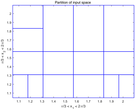
The image displays a 2D Cartesian coordinate plot showing a rectangular area that has been subdivided into smaller, non-uniform rectangular regions. The plot represents a mathematical or computational "partition of input space," where a continuous 2D domain is discretized into specific bounding boxes. The grid lines are solid blue, set against a white background.
### Components/Axes
**1. Header (Top Center)**
* **Title:** "Partition of input space"
**2. X-Axis (Bottom)**
* **Label:** $\pi/3 < x_1 < 2\pi/3$ (Centered below the axis).
* **Scale/Range:** The visual axis begins slightly before 1.1 and ends slightly after 2.0, corresponding to the mathematical range of approximately $[1.047, 2.094]$.
* **Tick Markers:** 1.1, 1.2, 1.3, 1.4, 1.5, 1.6, 1.7, 1.8, 1.9, 2 (Spaced evenly at 0.1 intervals).
**3. Y-Axis (Left)**
* **Label:** $\pi/3 < x_2 < 2\pi/3$ (Rotated 90 degrees counter-clockwise, centered left of the axis).
* **Scale/Range:** Identical to the X-axis, representing approximately $[1.047, 2.094]$.
* **Tick Markers:** 1.1, 1.2, 1.3, 1.4, 1.5, 1.6, 1.7, 1.8, 1.9, 2 (Spaced evenly at 0.1 intervals).
### Detailed Analysis
The main chart area consists of a bounding box defined by the limits $\pi/3$ and $2\pi/3$ on both axes. This space is divided by a series of orthogonal blue lines. Based on the axis labels and visual placement, these lines correspond to recursive bisections (midpoints) of the mathematical intervals.
**Primary Grid Lines (Spanning the entire width/height):**
* **Vertical Lines ($x_1$):**
* $x_1 \approx 1.31$ (Mathematically deduced as $5\pi/12$, the midpoint of $[\pi/3, \pi/2]$)
* $x_1 \approx 1.57$ (Mathematically deduced as $\pi/2$, the midpoint of $[\pi/3, 2\pi/3]$)
* $x_1 \approx 1.83$ (Mathematically deduced as $7\pi/12$, the midpoint of $[\pi/2, 2\pi/3]$)
* **Horizontal Lines ($x_2$):**
* $x_2 \approx 1.31$ (Mathematically deduced as $5\pi/12$)
* $x_2 \approx 1.57$ (Mathematically deduced as $\pi/2$)
**Secondary/Minor Grid Lines (Partial spans):**
* **Top-Left Region:** A horizontal line at $x_2 \approx 1.83$ ($7\pi/12$) splits the column where $x_1 < 1.31$ and $x_2 > 1.57$.
* **Bottom-Left Region:** A vertical line at $x_1 \approx 1.18$ (Mathematically deduced as $3\pi/8$, the midpoint of $[\pi/3, 5\pi/12]$) splits the box where $x_1 < 1.31$ and $x_2 < 1.31$.
* **Bottom-Right Region:** A vertical line at $x_1 \approx 1.96$ (Mathematically deduced as $5\pi/8$, the midpoint of $[7\pi/12, 2\pi/3]$) splits the box where $x_1 > 1.83$ and $x_2 < 1.31$.
**Resulting Partitions:**
The space is divided into 15 distinct rectangular regions of varying sizes. The largest regions are located in the upper-right quadrant, while the smallest, most densely partitioned regions are located in the bottom-left, bottom-right, and top-left extremities.
### Key Observations
* **Non-Uniformity:** The grid is not a standard, equally spaced mesh. It exhibits localized refinement.
* **Recursive Bisection Pattern:** The placement of the lines strongly suggests a binary space partitioning algorithm. The domain is split in half ($\pi/2$), then those halves are split ($5\pi/12$, $7\pi/12$), and specific sub-regions are split again ($3\pi/8$, $5\pi/8$).
* **Asymmetry:** While the primary vertical lines divide the space into four columns, the horizontal lines only divide it into three main rows, with further subdivision only occurring in specific localized boxes.
### Interpretation
This image demonstrates a **spatially adaptive partitioning strategy**, commonly used in computational mathematics, machine learning, and numerical analysis.
* **Underlying Function Behavior:** In techniques like Adaptive Mesh Refinement (AMR) for solving partial differential equations, or in decision tree algorithms (like k-d trees or CART), a space is subdivided more finely in areas where the underlying data or function is complex, highly variable, or contains steep gradients. Conversely, areas with large, undivided rectangles (like the center and top-right) suggest that the underlying function is relatively smooth, uniform, or of less interest in those regions.
* **Algorithmic Logic:** The strict adherence to midpoints (bisections of intervals based on fractions of $\pi$) indicates a programmatic, recursive algorithm rather than arbitrary manual drawing. The algorithm evaluates a region, determines if an error threshold or variance limit is exceeded, and if so, splits the region in half along one or both axes.
* **Focus Areas:** The higher density of partitions along the bottom edge ($x_2 < 1.31$) and the top-left corner indicates that the system required higher resolution or encountered more complexity in these specific boundary areas of the input space.