\n
## Diagram: Partition of Input Space
### Overview
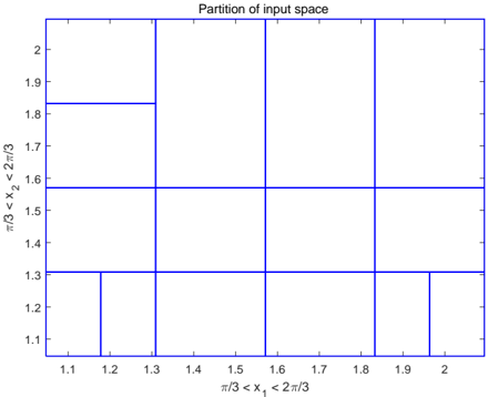
The image depicts a grid-like partition of a two-dimensional input space. The space is defined by the ranges of two variables, x₁ and x₂, both constrained between π/3 and 2π/3. The diagram visually represents a division of this space into rectangular regions.
### Components/Axes
* **Title:** "Partition of input space" - positioned at the top-center of the image.
* **X-axis Label:** "π/3 < x₁ < 2π/3" - located at the bottom of the image. The axis ranges from approximately 1.1 to 2.0.
* **Y-axis Label:** "π/3 < x₂ < 2π/3" - located on the left side of the image. The axis ranges from approximately 1.1 to 2.0.
* **Grid Lines:** A series of horizontal and vertical blue lines create a grid, dividing the space into rectangular cells. The lines are evenly spaced.
### Detailed Analysis
The diagram shows a 6x6 grid. The x-axis is divided into six equal segments, with markers at approximately 1.1, 1.2, 1.3, 1.4, 1.5, 1.6, 1.7, 1.8, 1.9, and 2.0. The y-axis is similarly divided into six equal segments, with markers at approximately 1.1, 1.2, 1.3, 1.4, 1.5, 1.6, 1.7, 1.8, 1.9, and 2.0.
The grid is formed by the intersection of these horizontal and vertical lines. Each cell represents a specific region within the defined input space. The grid is symmetrical.
### Key Observations
The diagram does not contain any data points or values *within* the grid cells. It simply illustrates a partitioning of the input space. The grid is uniform, suggesting equal division of the space.
### Interpretation
This diagram likely represents a discretization of a continuous input space for some computational or analytical purpose. The partitioning could be used for:
* **Quantization:** Mapping continuous values of x₁ and x₂ to discrete grid cells.
* **Classification:** Assigning data points to specific regions based on their x₁ and x₂ values.
* **Sampling:** Selecting representative points from each grid cell for analysis.
* **Feature Engineering:** Creating new features based on the grid cell a data point falls into.
The fact that the ranges for both x₁ and x₂ are identical (π/3 to 2π/3) suggests that the two variables are treated equally in this partitioning scheme. The diagram itself doesn't reveal the *purpose* of this partitioning, only *how* it is done. It is a visual representation of a mathematical space being divided into discrete regions.