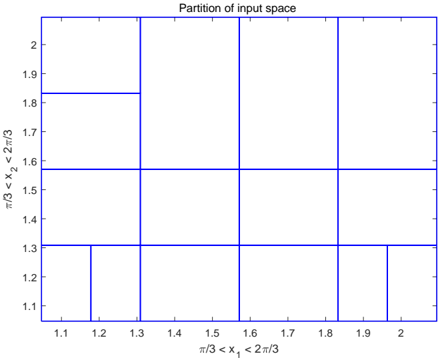
## Partition Diagram: Input Space Discretization ### Overview The image displays a 2D partition diagram titled "Partition of input space." It illustrates a rectangular domain divided into a non-uniform grid of smaller rectangular cells. The diagram is a technical visualization, likely representing a discretization scheme for numerical analysis, computational geometry, or machine learning feature space. ### Components/Axes * **Title:** "Partition of input space" (centered at the top). * **X-Axis:** * **Label:** `π/3 < x₁ < 2π/3` (positioned below the axis). * **Scale:** Linear, with major tick marks and numerical labels at `1.1, 1.2, 1.3, 1.4, 1.5, 1.6, 1.7, 1.8, 1.9, 2`. * **Range:** The visible axis spans from approximately `1.05` to `2.05`. The label indicates the theoretical domain is from `π/3` (≈1.047) to `2π/3` (≈2.094). * **Y-Axis:** * **Label:** `π/3 < x₂ < 2π/3` (positioned to the left, rotated 90 degrees). * **Scale:** Linear, with major tick marks and numerical labels at `1.1, 1.2, 1.3, 1.4, 1.5, 1.6, 1.7, 1.8, 1.9, 2`. * **Range:** Identical to the x-axis, from approximately `1.05` to `2.05`. * **Grid Lines:** The domain is partitioned by a set of vertical and horizontal blue lines. The lines are not uniformly spaced, creating cells of varying sizes. ### Detailed Analysis The partition is defined by the following set of vertical and horizontal lines: * **Vertical Lines (x-coordinates):** `1.1, 1.2, 1.3, 1.4, 1.5, 1.6, 1.7, 1.8, 1.9, 2.0` * **Horizontal Lines (y-coordinates):** `1.1, 1.2, 1.3, 1.4, 1.5, 1.6, 1.7, 1.8, 1.9, 2.0` However, not all lines extend across the entire domain. The grid is **non-uniform**, meaning some lines are omitted in certain regions, merging adjacent potential cells into larger rectangles. This creates a structured but adaptive mesh. **Spatial Structure (from bottom-left corner moving right and up):** 1. **Bottom-Left Corner:** A small cell defined by `x ∈ [1.1, 1.2]`, `y ∈ [1.1, 1.3]`. The horizontal line at `y=1.2` is absent in this column. 2. **Left Column (x from 1.1 to 1.3):** * A large vertical cell spanning `x ∈ [1.1, 1.3]`, `y ∈ [1.3, 1.8]`. The vertical line at `x=1.2` is absent in this row band. * A top-left cell spanning `x ∈ [1.1, 1.3]`, `y ∈ [1.8, 2.0]`. 3. **Column (x from 1.2 to 1.3):** Two small cells at the bottom: `y ∈ [1.1, 1.2]` and `y ∈ [1.2, 1.3]`. 4. **Remaining Columns (x from 1.3 to 2.0):** The grid becomes more regular. Each column from `1.3` to `2.0` is divided into three horizontal bands by the lines at `y=1.3` and `y=1.8`, creating cells for `y ∈ [1.1, 1.3]`, `y ∈ [1.3, 1.8]`, and `y ∈ [1.8, 2.0]`. The horizontal line at `y=1.2` is present only in the column `x ∈ [1.2, 1.3]`. ### Key Observations * **Non-Uniform Refinement:** The partition is finest (smallest cells) in the bottom-left corner (`x` near `1.1-1.2`, `y` near `1.1-1.3`) and along the bottom edge for `x > 1.2`. It is coarsest (largest cells) in the central-left region (`x ∈ [1.1, 1.3]`, `y ∈ [1.3, 1.8]`). * **Axis Label Discrepancy:** The axis labels define the domain using `π/3` and `2π/3`, but the grid lines and tick marks use decimal approximations. The grid does not align perfectly with the symbolic boundaries (e.g., the first grid line is at `1.1`, not `π/3 ≈ 1.047`). * **Structural Pattern:** The partition appears to follow a rule where refinement is concentrated near the lower bounds of both variables (`x₁` and `x₂` near `π/3`). ### Interpretation This diagram visualizes a **structured, adaptive discretization** of a 2D input space. The non-uniform grid suggests that the underlying problem or function being analyzed has higher complexity, variability, or requires greater resolution in specific regions—particularly where both input variables are near their lower limit (`π/3`). * **Purpose:** Such partitions are common in numerical methods like finite element analysis, adaptive mesh refinement for solving PDEs, or in machine learning for creating decision tree splits or binning strategies in regions of high data density or nonlinearity. * **Relationship Between Elements:** The axes define the continuous domain. The grid lines represent the boundaries of discrete sub-domains (cells). The variation in cell size indicates an **adaptive strategy**, allocating more computational resources (smaller cells) to areas deemed more important or difficult. * **Notable Anomaly:** The primary anomaly is the deliberate omission of certain grid lines (e.g., `x=1.2` for `y > 1.3`, `y=1.2` for `x < 1.3`), which is the core feature defining the adaptive nature of the partition. This is not an error but a design choice. * **Underlying Logic:** The pattern implies that the "input space" is not treated uniformly. The region near `(x₁, x₂) = (π/3, π/3)` is considered critical, warranting a finer mesh, while the central region `(x₁, x₂) ≈ (1.2, 1.55)` is considered less critical, allowing for a coarser representation. This could be due to boundary layer effects, singularities, or higher gradient magnitudes near the lower bounds.