## Grid Partition Diagram: Partition of Input Space
### Overview
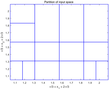
The image depicts a 2D grid partitioning an input space defined by two variables, \( x_1 \) and \( x_2 \). The grid is divided into 12 rectangular regions using blue lines, with labeled axes and coordinate markers. The structure suggests a systematic discretization of the input domain for analysis or computational purposes.
### Components/Axes
- **Title**: "Partition of input space" (centered at the top).
- **X-axis**: Labeled \( \pi/3 < x_1 < 2\pi/3 \), with numerical markers from 1.1 to 2.0 in increments of 0.1.
- **Y-axis**: Labeled \( \pi/3 < x_2 < 2\pi/3 \), with numerical markers from 1.1 to 2.0 in increments of 0.1.
- **Grid Lines**: Blue vertical and horizontal lines dividing the space into 12 regions.
- **Region Coordinates**: Each region is annotated with approximate coordinate pairs (e.g., (1.1, 1.1), (1.2, 1.2), etc.), positioned near the bottom-left corner of each cell.
### Detailed Analysis
- **Grid Structure**:
- The grid spans \( x_1 \in [1.1, 2.0] \) and \( x_2 \in [1.1, 2.0] \).
- Vertical lines at \( x_1 = 1.1, 1.2, ..., 2.0 \).
- Horizontal lines at \( x_2 = 1.1, 1.2, ..., 2.0 \).
- Regions are labeled with coordinate pairs (e.g., (1.1, 1.1) for the bottom-left cell, (1.9, 1.9) for the top-right cell).
- **Approximate Boundaries**:
- Each cell spans approximately 0.1 units in both \( x_1 \) and \( x_2 \).
- Example: The cell labeled (1.3, 1.3) spans \( x_1 \in [1.3, 1.4] \) and \( x_2 \in [1.3, 1.4] \).
### Key Observations
1. **Uniform Partitioning**: The grid is evenly spaced, with consistent intervals of 0.1 units along both axes.
2. **Coordinate Labels**: All regions are labeled with their approximate coordinate pairs, though the exact boundaries are not explicitly marked.
3. **Symmetry**: The grid is symmetric about the diagonal \( x_1 = x_2 \), suggesting a balanced partitioning of the input space.
### Interpretation
This diagram represents a discretized input space for a function or system, where each cell corresponds to a specific range of \( x_1 \) and \( x_2 \) values. The uniform grid implies a methodical approach to exploring the input domain, likely for numerical simulations, optimization, or machine learning tasks. The absence of data points or color gradients suggests the grid is a structural framework rather than a representation of measured or computed values. The labels \( \pi/3 < x_1 < 2\pi/3 \) and \( \pi/3 < x_2 < 2\pi/3 \) indicate the input variables are constrained to angular ranges, possibly related to trigonometric or periodic systems. The partitioning could facilitate stepwise analysis, such as evaluating a function’s behavior across discrete intervals or training a model on segmented data.