TECHNICAL ASSET FINGERPRINT
d6a6e3fb0ee43ec61231ee38
Click to view fullscreen
Press ESC or click to close
FOUND IN PAPERS
EXPERT: healer-alpha-free VERSION 1
RUNTIME: free/openrouter/healer-alpha
INTEL_VERIFIED
## [Multi-Panel Box Plot]: Causal Effect (ATE) Comparison Across Six Scenarios
### Overview
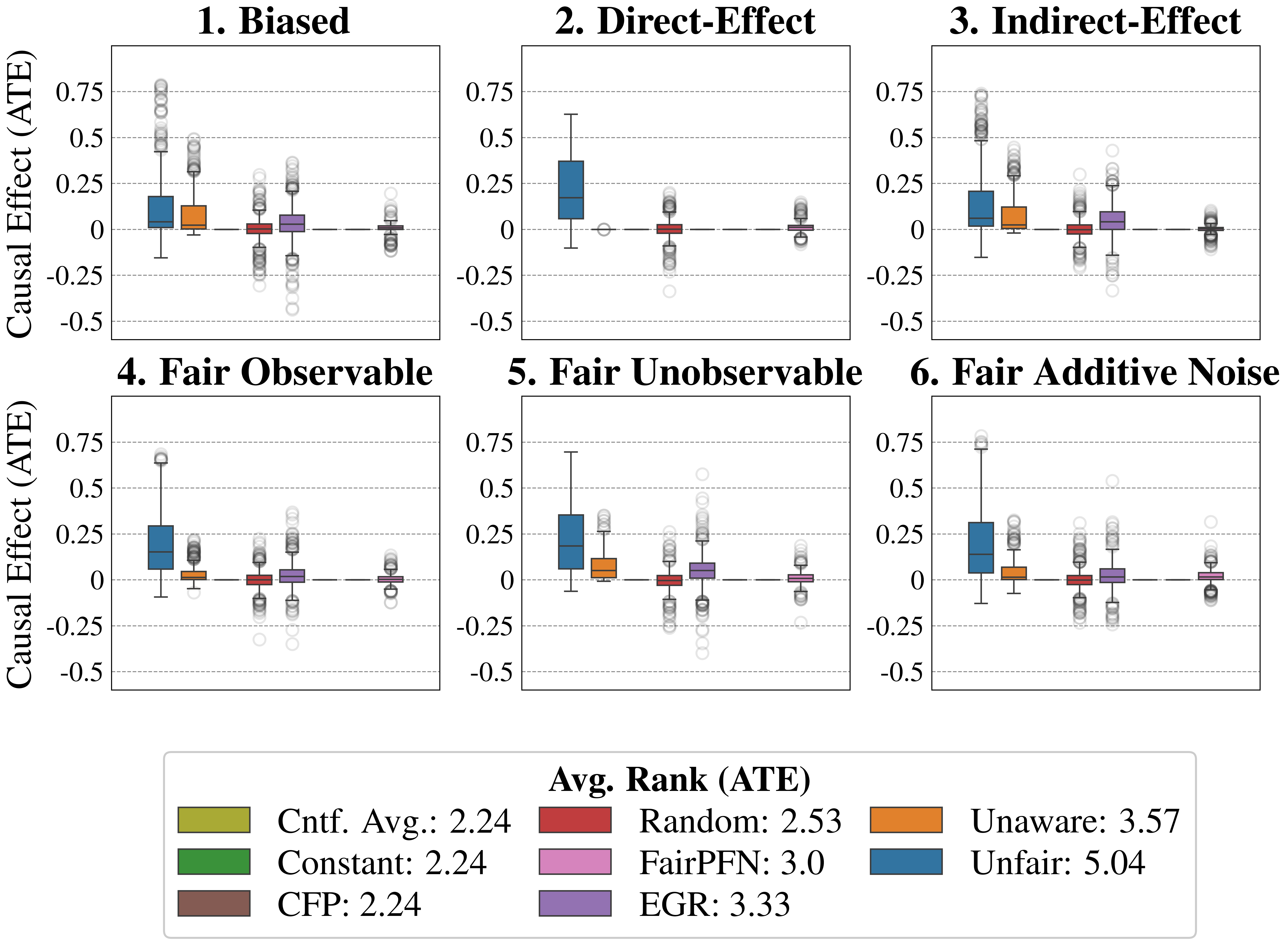
The image displays a 2x3 grid of six box plots, each comparing the distribution of the Average Treatment Effect (ATE) for eight different methods under distinct causal scenarios. The overall purpose is to evaluate and compare the performance (in terms of estimated causal effect) of various fairness-aware and baseline methods. A legend at the bottom provides color coding and an average rank for each method.
### Components/Axes
* **Chart Type:** Six separate box plot panels.
* **Y-Axis (All Panels):** Labeled "Causal Effect (ATE)". The scale ranges from -0.5 to 0.75, with major gridlines at intervals of 0.25 (-0.5, -0.25, 0, 0.25, 0.5, 0.75).
* **Panel Titles (Top Row, Left to Right):**
1. Biased
2. Direct-Effect
3. Indirect-Effect
* **Panel Titles (Bottom Row, Left to Right):**
4. Fair Observable
5. Fair Unobservable
6. Fair Additive Noise
* **Legend (Bottom Center):** Titled "Avg. Rank (ATE)". It lists eight methods with associated color swatches and their average rank (lower is better).
* **Ctf. Avg.:** Olive green, Avg. Rank: 2.24
* **Constant:** Forest green, Avg. Rank: 2.24
* **CFP:** Brown, Avg. Rank: 2.24
* **Random:** Red, Avg. Rank: 2.53
* **FairPFN:** Pink, Avg. Rank: 3.0
* **EGR:** Purple, Avg. Rank: 3.33
* **Unaware:** Orange, Avg. Rank: 3.57
* **Unfair:** Blue, Avg. Rank: 5.04
### Detailed Analysis
Each panel contains eight box plots, one per method, ordered consistently from left to right: Unfair (blue), Unaware (orange), Random (red), FairPFN (pink), EGR (purple), Ctf. Avg. (olive), Constant (green), CFP (brown). The box represents the interquartile range (IQR), the line inside is the median, whiskers extend to 1.5x IQR, and circles are outliers.
**Panel 1: Biased**
* **Unfair (Blue):** Median ~0.05, IQR spans ~0 to ~0.2, whiskers from ~-0.15 to ~0.45. Many high outliers up to ~0.75.
* **Unaware (Orange):** Median ~0.05, IQR ~0 to ~0.15, whiskers ~-0.05 to ~0.3. Outliers up to ~0.5.
* **Random (Red):** Median ~0, very narrow IQR centered on 0. Whiskers ~-0.05 to ~0.05. Outliers from ~-0.25 to ~0.25.
* **FairPFN (Pink):** Median ~0, IQR ~-0.05 to ~0.05. Whiskers ~-0.15 to ~0.15. Many outliers from ~-0.5 to ~0.35.
* **EGR (Purple):** Median ~0, IQR ~-0.05 to ~0.05. Whiskers ~-0.1 to ~0.1. Outliers from ~-0.4 to ~0.3.
* **Ctf. Avg., Constant, CFP (Olive, Green, Brown):** All distributions are extremely tight, centered at 0 with minimal spread and few outliers near 0.
**Panel 2: Direct-Effect**
* **Unfair (Blue):** Median ~0.2, IQR ~0.05 to ~0.35. Whiskers ~-0.1 to ~0.65. No visible outliers.
* **Unaware (Orange):** Appears as a single point or extremely narrow distribution at 0.
* **Random (Red):** Median ~0, narrow IQR. Whiskers ~-0.05 to ~0.05. Outliers from ~-0.35 to ~0.2.
* **FairPFN (Pink):** Median ~0, narrow IQR. Whiskers ~-0.05 to ~0.05. Outliers from ~-0.1 to ~0.1.
* **EGR (Purple):** Median ~0, narrow IQR. Whiskers ~-0.05 to ~0.05. Outliers from ~-0.1 to ~0.1.
* **Ctf. Avg., Constant, CFP:** Extremely tight distributions at 0.
**Panel 3: Indirect-Effect**
* **Unfair (Blue):** Median ~0.05, IQR ~0 to ~0.2. Whiskers ~-0.15 to ~0.45. Many high outliers up to ~0.75.
* **Unaware (Orange):** Median ~0.05, IQR ~0 to ~0.1. Whiskers ~-0.05 to ~0.2. Outliers up to ~0.4.
* **Random (Red):** Median ~0, narrow IQR. Whiskers ~-0.05 to ~0.05. Outliers from ~-0.2 to ~0.2.
* **FairPFN (Pink):** Median ~0, IQR ~-0.05 to ~0.05. Whiskers ~-0.15 to ~0.15. Outliers from ~-0.3 to ~0.4.
* **EGR (Purple):** Median ~0, IQR ~-0.05 to ~0.05. Whiskers ~-0.1 to ~0.1. Outliers from ~-0.25 to ~0.25.
* **Ctf. Avg., Constant, CFP:** Extremely tight distributions at 0.
**Panel 4: Fair Observable**
* **Unfair (Blue):** Median ~0.15, IQR ~0.05 to ~0.3. Whiskers ~-0.1 to ~0.65. One high outlier ~0.65.
* **Unaware (Orange):** Median ~0.05, IQR ~0 to ~0.1. Whiskers ~-0.05 to ~0.15. Outliers up to ~0.25.
* **Random (Red):** Median ~0, narrow IQR. Whiskers ~-0.05 to ~0.05. Outliers from ~-0.3 to ~0.2.
* **FairPFN (Pink):** Median ~0, IQR ~-0.05 to ~0.05. Whiskers ~-0.15 to ~0.15. Outliers from ~-0.4 to ~0.35.
* **EGR (Purple):** Median ~0, IQR ~-0.05 to ~0.05. Whiskers ~-0.1 to ~0.1. Outliers from ~-0.3 to ~0.25.
* **Ctf. Avg., Constant, CFP:** Extremely tight distributions at 0.
**Panel 5: Fair Unobservable**
* **Unfair (Blue):** Median ~0.2, IQR ~0.05 to ~0.35. Whiskers ~-0.05 to ~0.7. No visible outliers.
* **Unaware (Orange):** Median ~0.05, IQR ~0 to ~0.1. Whiskers ~-0.05 to ~0.15. Outliers up to ~0.35.
* **Random (Red):** Median ~0, narrow IQR. Whiskers ~-0.05 to ~0.05. Outliers from ~-0.25 to ~0.25.
* **FairPFN (Pink):** Median ~0, IQR ~-0.05 to ~0.05. Whiskers ~-0.15 to ~0.15. Outliers from ~-0.4 to ~0.6.
* **EGR (Purple):** Median ~0, IQR ~-0.05 to ~0.05. Whiskers ~-0.1 to ~0.1. Outliers from ~-0.25 to ~0.25.
* **Ctf. Avg., Constant, CFP:** Extremely tight distributions at 0.
**Panel 6: Fair Additive Noise**
* **Unfair (Blue):** Median ~0.15, IQR ~0.05 to ~0.3. Whiskers ~-0.15 to ~0.75. One high outlier ~0.75.
* **Unaware (Orange):** Median ~0.05, IQR ~0 to ~0.1. Whiskers ~-0.05 to ~0.15. Outliers up to ~0.3.
* **Random (Red):** Median ~0, narrow IQR. Whiskers ~-0.05 to ~0.05. Outliers from ~-0.25 to ~0.3.
* **FairPFN (Pink):** Median ~0, IQR ~-0.05 to ~0.05. Whiskers ~-0.15 to ~0.15. Outliers from ~-0.25 to ~0.55.
* **EGR (Purple):** Median ~0, IQR ~-0.05 to ~0.05. Whiskers ~-0.1 to ~0.1. Outliers from ~-0.25 to ~0.25.
* **Ctf. Avg., Constant, CFP:** Extremely tight distributions at 0.
### Key Observations
1. **Consistent Hierarchy:** Across all six scenarios, the **Unfair** method (blue) consistently shows the highest median ATE and the largest spread (variance). The **Unaware** method (orange) is typically second highest. Methods like **Constant**, **CFP**, and **Ctf. Avg.** are consistently centered at zero with negligible variance.
2. **Scenario Impact:** The "Direct-Effect" and "Fair Unobservable" scenarios appear to induce the largest positive ATE for the Unfair method (medians ~0.2). The "Biased" and "Indirect-Effect" scenarios show more outliers for the Unfair method.
3. **Fairness Methods:** Fairness-aware methods (**Random**, **FairPFN**, **EGR**) generally have medians near zero, similar to the constant baselines, but exhibit more variance and outliers, especially **FairPFN**.
4. **Ranking Confirmation:** The visual data aligns with the legend's average ranks. The Unfair method (rank 5.04) has the worst (highest) values, while the tied methods with rank 2.24 (Ctf. Avg., Constant, CFP) are the most stable at zero.
### Interpretation
This visualization is a comparative analysis of algorithmic fairness in causal inference. The "Causal Effect (ATE)" likely represents a measure of bias or disparate impact. The six panels represent different data-generating processes or fairness constraints imposed on the underlying model.
* **What the data suggests:** The "Unfair" method, which presumably ignores fairness constraints, produces the largest and most variable estimated causal effects (biases). The "Unaware" method, which may be blind to sensitive attributes, still shows significant bias. In contrast, methods explicitly designed for fairness (FairPFN, EGR) or simple baselines (Constant, CFP) successfully drive the estimated ATE towards zero, indicating they are mitigating the measured bias.
* **Relationship between elements:** The box plots allow for a direct comparison of the *distribution* of outcomes, not just point estimates. The tight clustering of the constant methods at zero serves as a control, showing what a perfectly "fair" (or null) effect looks like. The spread of the other methods indicates their sensitivity to the underlying scenario.
* **Notable patterns:** The key takeaway is the trade-off between variance and bias. The unfair/unaware methods have high bias (non-zero median ATE) but also high variance. The fairness-aware methods achieve low bias (median ~0) but introduce more variance into the estimates compared to the rigid constant baselines. The "Direct-Effect" scenario seems to be the most challenging for the unfair method, producing the highest median bias.
DECODING INTELLIGENCE...