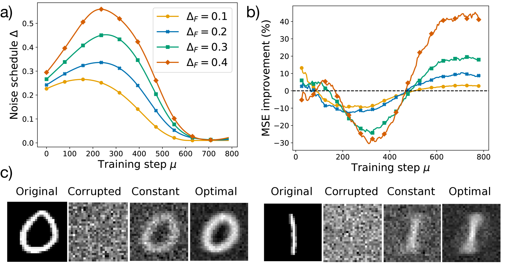
## Chart/Diagram Type: Multi-Panel Figure ### Overview The image consists of three subfigures labeled a), b), and c). Subfigures a) and b) are line plots showing the relationship between training step and noise schedule, and training step and MSE improvement, respectively. Subfigure c) displays example images of digits in original, corrupted, constant, and optimal states. ### Components/Axes **Subfigure a): Noise Schedule vs. Training Step** * **Title:** a) * **X-axis:** Training step μ * Scale: 0 to 800, with increments of 100. * **Y-axis:** Noise schedule Δ * Scale: 0.0 to 0.5, with increments of 0.1. * **Legend:** Located in the top-right corner of the plot. * Yellow: ΔF = 0.1 * Blue: ΔF = 0.2 * Green: ΔF = 0.3 * Orange: ΔF = 0.4 **Subfigure b): MSE Improvement vs. Training Step** * **Title:** b) * **X-axis:** Training step μ * Scale: 0 to 800, with increments of 200. * **Y-axis:** MSE improvement (%) * Scale: -30 to 40, with increments of 10. * **Horizontal dashed line:** Represents 0% MSE improvement. * **Legend:** (Inferred from Subfigure a) * Yellow: ΔF = 0.1 * Blue: ΔF = 0.2 * Green: ΔF = 0.3 * Orange: ΔF = 0.4 **Subfigure c): Example Images** * **Labels:** * Original * Corrupted * Constant * Optimal * **Images:** Two rows of images, each row containing the four states (Original, Corrupted, Constant, Optimal) of a digit. The top row shows the digit "0", and the bottom row shows the digit "1". ### Detailed Analysis **Subfigure a): Noise Schedule vs. Training Step** * **Yellow (ΔF = 0.1):** Starts at approximately 0.23, increases to a peak around 0.27 at a training step of approximately 200, then decreases to approximately 0.02 at a training step of 700-800. * **Blue (ΔF = 0.2):** Starts at approximately 0.26, increases to a peak around 0.33 at a training step of approximately 200, then decreases to approximately 0.02 at a training step of 700-800. * **Green (ΔF = 0.3):** Starts at approximately 0.28, increases to a peak around 0.44 at a training step of approximately 250, then decreases to approximately 0.02 at a training step of 700-800. * **Orange (ΔF = 0.4):** Starts at approximately 0.22, increases to a peak around 0.56 at a training step of approximately 250, then decreases to approximately 0.02 at a training step of 700-800. **Subfigure b): MSE Improvement vs. Training Step** * **Yellow (ΔF = 0.1):** Starts at approximately 13%, decreases to a minimum of approximately -12% at a training step of approximately 350, then increases to approximately 3% at a training step of 800. * **Blue (ΔF = 0.2):** Starts at approximately 4%, decreases to a minimum of approximately -15% at a training step of approximately 350, then increases to approximately 9% at a training step of 800. * **Green (ΔF = 0.3):** Starts at approximately 7%, decreases to a minimum of approximately -27% at a training step of approximately 350, then increases to approximately 17% at a training step of 800. * **Orange (ΔF = 0.4):** Starts at approximately -5%, decreases to a minimum of approximately -28% at a training step of approximately 350, then increases to approximately 38% at a training step of 800. **Subfigure c): Example Images** * The "Original" images are clear representations of the digits "0" and "1". * The "Corrupted" images show the digits with added noise, making them difficult to recognize. * The "Constant" images show the digits after applying a constant noise schedule. * The "Optimal" images show the digits after applying an optimized noise schedule, resulting in clearer representations compared to the "Constant" images. ### Key Observations * In subfigure a), as ΔF increases, the peak of the noise schedule also increases. All noise schedules converge to a similar low value at higher training steps. * In subfigure b), higher ΔF values lead to greater MSE improvement at higher training steps, but also to a greater decrease in MSE improvement at lower training steps. * In subfigure c), the "Optimal" images are visually better reconstructions of the original digits compared to the "Constant" images. ### Interpretation The data suggests that the noise schedule (Δ) plays a crucial role in the training process. Higher values of ΔF lead to a more aggressive noise schedule, which initially degrades performance (negative MSE improvement) but ultimately leads to better performance (positive MSE improvement) at later stages of training. The example images in subfigure c) visually confirm that the optimized noise schedule results in better image reconstruction compared to a constant noise schedule. The relationship between ΔF and MSE improvement indicates a trade-off between initial performance and final performance, suggesting that the optimal ΔF value depends on the specific training goals and constraints.

\n ## Charts/Graphs: Noise Schedule and MSE Improvement with Training ### Overview The image presents three distinct visualizations: a line chart (a) showing noise schedule delta (Δ) versus training step (μ) for different ΔF values, another line chart (b) displaying MSE improvement (%) against training step (μ) also for different ΔF values, and a series of images (c) illustrating the reconstruction of two different shapes (a circle and a line) under various noise conditions (Original, Corrupted, Constant, Optimal). ### Components/Axes **Chart a): Noise Schedule Δ vs. Training Step μ** * **X-axis:** Training step μ (ranging from approximately 0 to 800). * **Y-axis:** Noise schedule Δ (ranging from approximately 0 to 0.5). * **Legend:** * ΔF = 0.1 (represented by a yellow line) * ΔF = 0.2 (represented by a blue line) * ΔF = 0.3 (represented by a green line) * ΔF = 0.4 (represented by a red line) **Chart b): MSE Improvement (%) vs. Training Step μ** * **X-axis:** Training step μ (ranging from approximately 0 to 800). * **Y-axis:** MSE improvement (%) (ranging from approximately -30% to 40%). * **Legend:** (Colors correspond to Chart a) * ΔF = 0.1 (represented by a yellow line) * ΔF = 0.2 (represented by a blue line) * ΔF = 0.3 (represented by a green line) * ΔF = 0.4 (represented by a red line) **Images c): Reconstruction Examples** * Columns: Original, Corrupted, Constant, Optimal. * Rows: Two different shapes (a circle and a vertical line). ### Detailed Analysis or Content Details **Chart a): Noise Schedule Δ vs. Training Step μ** * **ΔF = 0.1 (Yellow):** Starts at approximately 0.25, rises to a peak of around 0.45 at μ ≈ 200, then declines to approximately 0.02 by μ = 800. * **ΔF = 0.2 (Blue):** Starts at approximately 0.25, rises to a peak of around 0.4 at μ ≈ 150, then declines to approximately 0.01 by μ = 800. * **ΔF = 0.3 (Green):** Starts at approximately 0.25, rises to a peak of around 0.35 at μ ≈ 100, then declines to approximately 0.01 by μ = 800. * **ΔF = 0.4 (Red):** Starts at approximately 0.25, rises to a peak of around 0.5 at μ ≈ 50, then declines to approximately 0.01 by μ = 800. **Chart b): MSE Improvement (%) vs. Training Step μ** * **ΔF = 0.1 (Yellow):** Initially fluctuates around 0%, then increases steadily from μ ≈ 400, reaching approximately 30% at μ = 800. * **ΔF = 0.2 (Blue):** Initially fluctuates around 0%, then increases steadily from μ ≈ 400, reaching approximately 35% at μ = 800. * **ΔF = 0.3 (Green):** Initially fluctuates around 0%, then increases steadily from μ ≈ 400, reaching approximately 25% at μ = 800. * **ΔF = 0.4 (Red):** Shows a significant initial dip to approximately -30% at μ ≈ 100, then recovers and increases steadily from μ ≈ 400, reaching approximately 10% at μ = 800. **Images c): Reconstruction Examples** * **Circle:** * Original: Clear circle. * Corrupted: Noisy, distorted circle. * Constant: Partially reconstructed circle with significant noise. * Optimal: Well-reconstructed circle with minimal noise. * **Line:** * Original: Clear vertical line. * Corrupted: Noisy, distorted line. * Constant: Partially reconstructed line with significant noise. * Optimal: Well-reconstructed line with minimal noise. ### Key Observations * The noise schedule (Chart a) peaks early in training and then decays for all ΔF values. * Higher ΔF values (0.3 and 0.4) initially exhibit lower MSE improvement (Chart b) but show recovery during later training stages. * The "Optimal" reconstruction in images (c) demonstrates the effectiveness of the training process in removing noise and recovering the original shapes. * The "Constant" reconstruction shows that a fixed noise schedule is less effective than the dynamic schedule. ### Interpretation The data suggests that a dynamic noise schedule, controlled by ΔF, is crucial for effective training. The initial peak in the noise schedule (Chart a) likely introduces sufficient stochasticity to prevent the model from getting stuck in local minima. The subsequent decay allows for refinement and convergence. The MSE improvement (Chart b) indicates that higher ΔF values may require longer training times to achieve optimal performance, as they initially lead to a larger error. The reconstruction examples (c) visually confirm the benefits of the optimal noise schedule in recovering the original data from noisy inputs. The initial dip in MSE for ΔF=0.4 suggests a period of instability or increased error before the model adapts and begins to improve. The consistent improvement of the "Optimal" reconstruction across both shapes indicates the robustness of the method.

## Line Charts and Image Comparison: Noise Schedule Optimization for Image Reconstruction ### Overview The image is a composite figure containing three panels labeled a), b), and c). Panels a) and b) are line charts plotting metrics against training steps for different noise schedule parameters. Panel c) provides a visual comparison of image reconstruction results. The overall subject appears to be the optimization of a noise schedule (Δ) during a training process to improve image reconstruction quality, measured by Mean Squared Error (MSE) improvement. ### Components/Axes **Panel a):** * **Chart Type:** Line chart. * **X-axis:** Label: "Training step μ". Scale: Linear, from 0 to 800, with major ticks every 100 steps. * **Y-axis:** Label: "Noise schedule Δ". Scale: Linear, from 0.0 to 0.5, with major ticks every 0.1. * **Legend:** Located in the top-right corner. Contains four entries, each corresponding to a different value of ΔF: * Yellow line with circle markers: ΔF = 0.1 * Blue line with 'x' markers: ΔF = 0.2 * Green line with square markers: ΔF = 0.3 * Orange line with diamond markers: ΔF = 0.4 **Panel b):** * **Chart Type:** Line chart. * **X-axis:** Label: "Training step μ". Scale: Linear, from 0 to 800, with major ticks every 200 steps. * **Y-axis:** Label: "MSE improvement (%)". Scale: Linear, from -30 to 40, with major ticks every 10%. A dashed horizontal line at 0% indicates the baseline. * **Legend:** Implicitly matches the legend from panel a) by color and marker style. The four lines correspond to the same ΔF values (0.1, 0.2, 0.3, 0.4). **Panel c):** * **Content:** Two sets of four grayscale images each, arranged in a 2x4 grid. * **Column Headers (Top Row):** "Original", "Corrupted", "Constant", "Optimal". These headers are repeated for the second set of images below. * **Image Set 1 (Left):** Shows the reconstruction of a handwritten digit "0". * **Image Set 2 (Right):** Shows the reconstruction of a handwritten digit "1". ### Detailed Analysis **Panel a) - Noise Schedule Δ vs. Training Step:** * **Trend Verification:** All four lines follow a similar inverted-U shape. They start at a moderate value, rise to a peak between steps 200-300, and then decay towards zero by step 800. * **Data Points (Approximate):** * **ΔF = 0.1 (Yellow):** Starts ~0.23, peaks ~0.27 at step ~250, decays to ~0.01 by step 800. * **ΔF = 0.2 (Blue):** Starts ~0.24, peaks ~0.34 at step ~250, decays to ~0.01 by step 800. * **ΔF = 0.3 (Green):** Starts ~0.27, peaks ~0.45 at step ~250, decays to ~0.02 by step 800. * **ΔF = 0.4 (Orange):** Starts ~0.29, peaks ~0.55 at step ~250, decays to ~0.02 by step 800. * **Key Observation:** Higher ΔF values result in a higher peak noise schedule Δ. The peak occurs at approximately the same training step (~250) for all series. **Panel b) - MSE Improvement (%) vs. Training Step:** * **Trend Verification:** All lines show a similar pattern: initial fluctuation near 0%, a significant dip into negative improvement (worsening) between steps 100-400, followed by a recovery and rise into positive improvement after step 400. * **Data Points (Approximate):** * **ΔF = 0.1 (Yellow):** Shows the smallest dip (~ -10% at step ~300) and the smallest final improvement (~ +3% at step 800). * **ΔF = 0.2 (Blue):** Dips to ~ -12% at step ~300, recovers to ~ +9% at step 800. * **ΔF = 0.3 (Green):** Dips to ~ -25% at step ~350, recovers strongly to ~ +18% at step 800. * **ΔF = 0.4 (Orange):** Shows the most extreme behavior. Dips deepest to ~ -30% at step ~350, then recovers most strongly, reaching ~ +42% at step 800. * **Key Observation:** There is a clear trade-off. Higher ΔF values cause a more severe temporary degradation in performance (deeper negative dip) but lead to a much greater final improvement in MSE. The crossover point to net positive improvement occurs later for higher ΔF (around step 450 for ΔF=0.4 vs. step 400 for ΔF=0.1). **Panel c) - Visual Reconstruction Comparison:** * **Content Details:** * **Original:** Clean, high-contrast images of digits "0" and "1". * **Corrupted:** The same digits heavily obscured by what appears to be dense, random noise. The digit structure is barely discernible. * **Constant:** Reconstructions using a "Constant" noise schedule (presumably ΔF=0 or a fixed value). The digits are recognizable but blurry and retain significant noise artifacts. * **Optimal:** Reconstructions using the optimized noise schedule (likely corresponding to the best-performing ΔF from the charts, e.g., ΔF=0.4). These images are noticeably sharper and clearer than the "Constant" versions, with better-defined edges and less background noise, closely resembling the "Original". ### Key Observations 1. **Parameter Sensitivity:** The system's performance is highly sensitive to the ΔF parameter. ΔF=0.4 yields the best final MSE improvement but at the cost of the worst mid-training performance. 2. **Training Phase Duality:** The training process exhibits two distinct phases: an initial "destructive" phase where performance worsens (negative MSE improvement), followed by a "constructive" phase where performance improves significantly. 3. **Visual-Quantitative Correlation:** The "Optimal" images in panel c) visually confirm the quantitative improvement shown in panel b). The superior sharpness of the "Optimal" reconstructions aligns with the high positive MSE improvement percentages for higher ΔF values. ### Interpretation The data demonstrates the effectiveness of a dynamically scheduled noise parameter (Δ) in an iterative image reconstruction or denoising task. The core insight is that **introducing more noise (higher ΔF) during the critical mid-training phase (around steps 200-400), while detrimental in the short term, ultimately guides the model to a better solution.** * **Peircean Investigation:** The charts suggest a causal relationship: the optimized noise schedule (panel a) is the cause, and the improved MSE (panel b) and visual quality (panel c) are the effects. The "Constant" schedule acts as a control, proving that the dynamic schedule is the key variable. * **Underlying Mechanism:** This pattern is characteristic of optimization processes that escape local minima. The initial performance dip may represent the model being pushed out of a suboptimal solution (a local minimum) by the increased noise. The subsequent recovery and strong improvement indicate the model finding a deeper, more robust minimum in the loss landscape. * **Practical Implication:** For practitioners, this indicates a trade-off between training stability and final performance. Choosing a higher ΔF requires patience through a period of apparent degradation but promises superior results. The optimal ΔF value (0.4 in this case) maximizes the final outcome, suggesting the system benefits from a more aggressive exploration of the solution space early in training.

## Line Graphs and Image Comparisons: Noise Schedule and MSE Improvement Analysis ### Overview The image contains three components: 1. **Part a**: A line graph showing noise schedule (Δ) across training steps (μ) for four ΔF values (0.1–0.4). 2. **Part b**: A line graph showing MSE improvement (%) across training steps (μ) for the same ΔF values. 3. **Part c**: Four grayscale images per scenario (Original, Corrupted, Constant, Optimal) for two datasets. --- ### Components/Axes #### Part a: Noise Schedule Graph - **Y-axis**: "Noise schedule Δ" (range: 0.0–0.5). - **X-axis**: "Training step μ" (range: 0–800). - **Legend**: - Orange (ΔF=0.1) - Blue (ΔF=0.2) - Green (ΔF=0.3) - Red (ΔF=0.4) - **Legend Position**: Top-right corner. #### Part b: MSE Improvement Graph - **Y-axis**: "MSE improvement (%)" (range: -30% to 40%). - **X-axis**: "Training step μ" (range: 0–800). - **Legend**: Same color coding as Part a. - **Dashed Line**: Horizontal reference at 0%. #### Part c: Image Comparisons - **Labels**: - Left to right: Original, Corrupted, Constant, Optimal. - **Images**: Grayscale, showing varying clarity and noise levels. --- ### Detailed Analysis #### Part a: Noise Schedule Trends - **ΔF=0.4 (Red)**: Starts highest (~0.5 at μ=0), peaks sharply at μ≈200, then declines steeply to ~0.05 by μ=800. - **ΔF=0.3 (Green)**: Begins at ~0.35, peaks at μ≈200 (~0.45), declines to ~0.05 by μ=800. - **ΔF=0.2 (Blue)**: Starts at ~0.25, peaks at μ≈200 (~0.3), declines to ~0.05 by μ=800. - **ΔF=0.1 (Orange)**: Starts at ~0.2, peaks at μ≈200 (~0.25), declines to ~0.05 by μ=800. - **Convergence**: All lines merge near μ=800, with ΔF=0.4 consistently highest until μ≈600. #### Part b: MSE Improvement Trends - **ΔF=0.4 (Red)**: Dips below -20% at μ≈200, rises sharply to ~40% by μ=800. - **ΔF=0.3 (Green)**: Starts at ~5%, dips to -15% at μ≈200, rises to ~25% by μ=800. - **ΔF=0.2 (Blue)**: Starts at ~0%, dips to -10% at μ≈200, rises to ~10% by μ=800. - **ΔF=0.1 (Orange)**: Starts at ~10%, dips to -5% at μ≈200, stabilizes near 0% by μ=800. - **Dashed Line**: All lines cross the 0% baseline between μ=200–400. #### Part c: Image Comparisons - **Original**: Clear, high-contrast shapes (e.g., "O" and "I"). - **Corrupted**: Pixelated, noisy, and distorted. - **Constant**: Slightly improved clarity but retains noise. - **Optimal**: Sharp, noise-reduced reconstructions matching the original. --- ### Key Observations 1. **Noise Schedule (Part a)**: - Higher ΔF values (e.g., 0.4) reduce noise faster but start with higher initial noise. - All ΔF values converge to similar noise levels by μ=800. 2. **MSE Improvement (Part b)**: - ΔF=0.4 achieves the highest improvement (~40%), while ΔF=0.1 shows minimal gains. - Improvement correlates with noise reduction: lower noise (higher ΔF) yields better MSE. 3. **Image Quality (Part c)**: - "Optimal" images align with higher ΔF values, showing clearer reconstructions. - "Corrupted" images match the noisy trends in Part a. --- ### Interpretation - **Noise vs. Performance**: Higher ΔF values (0.3–0.4) balance faster noise reduction with superior MSE improvement, suggesting optimal training schedules for these parameters. - **Training Dynamics**: The initial noise peak (μ≈200) may reflect a transient phase where the model adjusts to corruption before stabilizing. - **Visual Correlation**: The "Optimal" images in Part c directly reflect the noise reduction trends in Part a and MSE improvements in Part b, validating the graphs' accuracy. - **Anomalies**: ΔF=0.1 underperforms in both noise reduction and MSE, indicating suboptimal parameter settings. This analysis demonstrates that ΔF=0.4 provides the best trade-off between noise suppression and reconstruction fidelity, as evidenced by both quantitative metrics and qualitative image comparisons.