\n
## Charts/Graphs: Noise Schedule and MSE Improvement with Training
### Overview
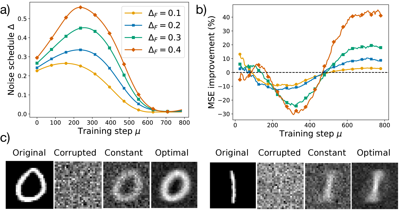
The image presents three distinct visualizations: a line chart (a) showing noise schedule delta (Δ) versus training step (μ) for different ΔF values, another line chart (b) displaying MSE improvement (%) against training step (μ) also for different ΔF values, and a series of images (c) illustrating the reconstruction of two different shapes (a circle and a line) under various noise conditions (Original, Corrupted, Constant, Optimal).
### Components/Axes
**Chart a): Noise Schedule Δ vs. Training Step μ**
* **X-axis:** Training step μ (ranging from approximately 0 to 800).
* **Y-axis:** Noise schedule Δ (ranging from approximately 0 to 0.5).
* **Legend:**
* ΔF = 0.1 (represented by a yellow line)
* ΔF = 0.2 (represented by a blue line)
* ΔF = 0.3 (represented by a green line)
* ΔF = 0.4 (represented by a red line)
**Chart b): MSE Improvement (%) vs. Training Step μ**
* **X-axis:** Training step μ (ranging from approximately 0 to 800).
* **Y-axis:** MSE improvement (%) (ranging from approximately -30% to 40%).
* **Legend:** (Colors correspond to Chart a)
* ΔF = 0.1 (represented by a yellow line)
* ΔF = 0.2 (represented by a blue line)
* ΔF = 0.3 (represented by a green line)
* ΔF = 0.4 (represented by a red line)
**Images c): Reconstruction Examples**
* Columns: Original, Corrupted, Constant, Optimal.
* Rows: Two different shapes (a circle and a vertical line).
### Detailed Analysis or Content Details
**Chart a): Noise Schedule Δ vs. Training Step μ**
* **ΔF = 0.1 (Yellow):** Starts at approximately 0.25, rises to a peak of around 0.45 at μ ≈ 200, then declines to approximately 0.02 by μ = 800.
* **ΔF = 0.2 (Blue):** Starts at approximately 0.25, rises to a peak of around 0.4 at μ ≈ 150, then declines to approximately 0.01 by μ = 800.
* **ΔF = 0.3 (Green):** Starts at approximately 0.25, rises to a peak of around 0.35 at μ ≈ 100, then declines to approximately 0.01 by μ = 800.
* **ΔF = 0.4 (Red):** Starts at approximately 0.25, rises to a peak of around 0.5 at μ ≈ 50, then declines to approximately 0.01 by μ = 800.
**Chart b): MSE Improvement (%) vs. Training Step μ**
* **ΔF = 0.1 (Yellow):** Initially fluctuates around 0%, then increases steadily from μ ≈ 400, reaching approximately 30% at μ = 800.
* **ΔF = 0.2 (Blue):** Initially fluctuates around 0%, then increases steadily from μ ≈ 400, reaching approximately 35% at μ = 800.
* **ΔF = 0.3 (Green):** Initially fluctuates around 0%, then increases steadily from μ ≈ 400, reaching approximately 25% at μ = 800.
* **ΔF = 0.4 (Red):** Shows a significant initial dip to approximately -30% at μ ≈ 100, then recovers and increases steadily from μ ≈ 400, reaching approximately 10% at μ = 800.
**Images c): Reconstruction Examples**
* **Circle:**
* Original: Clear circle.
* Corrupted: Noisy, distorted circle.
* Constant: Partially reconstructed circle with significant noise.
* Optimal: Well-reconstructed circle with minimal noise.
* **Line:**
* Original: Clear vertical line.
* Corrupted: Noisy, distorted line.
* Constant: Partially reconstructed line with significant noise.
* Optimal: Well-reconstructed line with minimal noise.
### Key Observations
* The noise schedule (Chart a) peaks early in training and then decays for all ΔF values.
* Higher ΔF values (0.3 and 0.4) initially exhibit lower MSE improvement (Chart b) but show recovery during later training stages.
* The "Optimal" reconstruction in images (c) demonstrates the effectiveness of the training process in removing noise and recovering the original shapes.
* The "Constant" reconstruction shows that a fixed noise schedule is less effective than the dynamic schedule.
### Interpretation
The data suggests that a dynamic noise schedule, controlled by ΔF, is crucial for effective training. The initial peak in the noise schedule (Chart a) likely introduces sufficient stochasticity to prevent the model from getting stuck in local minima. The subsequent decay allows for refinement and convergence. The MSE improvement (Chart b) indicates that higher ΔF values may require longer training times to achieve optimal performance, as they initially lead to a larger error. The reconstruction examples (c) visually confirm the benefits of the optimal noise schedule in recovering the original data from noisy inputs. The initial dip in MSE for ΔF=0.4 suggests a period of instability or increased error before the model adapts and begins to improve. The consistent improvement of the "Optimal" reconstruction across both shapes indicates the robustness of the method.