## Line Graphs and Image Comparisons: Noise Schedule and MSE Improvement Analysis
### Overview
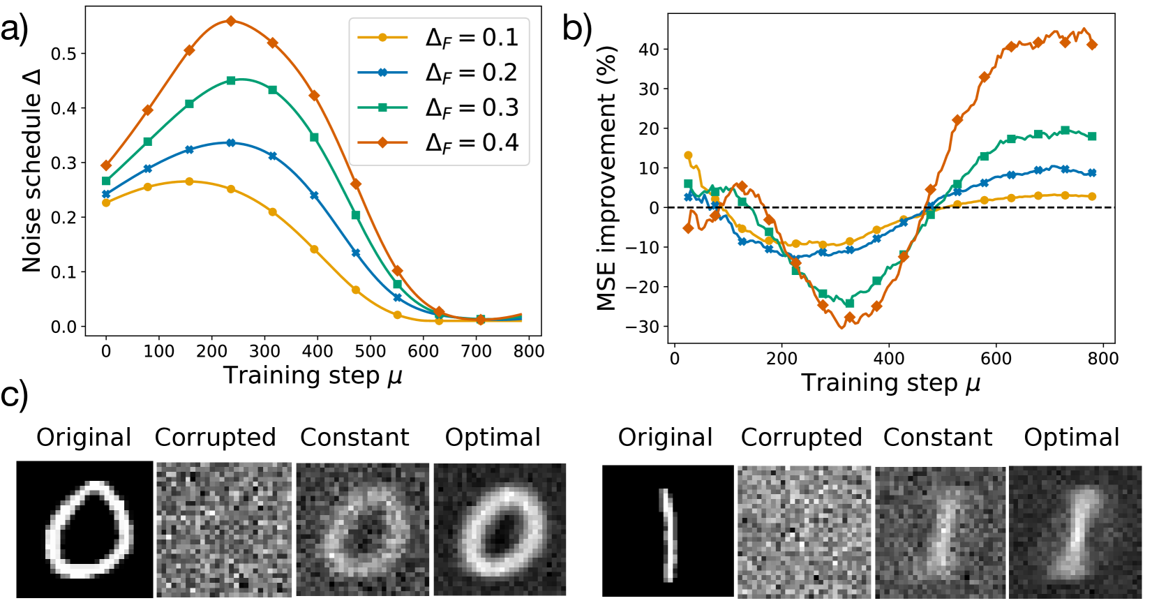
The image contains three components:
1. **Part a**: A line graph showing noise schedule (Δ) across training steps (μ) for four ΔF values (0.1–0.4).
2. **Part b**: A line graph showing MSE improvement (%) across training steps (μ) for the same ΔF values.
3. **Part c**: Four grayscale images per scenario (Original, Corrupted, Constant, Optimal) for two datasets.
---
### Components/Axes
#### Part a: Noise Schedule Graph
- **Y-axis**: "Noise schedule Δ" (range: 0.0–0.5).
- **X-axis**: "Training step μ" (range: 0–800).
- **Legend**:
- Orange (ΔF=0.1)
- Blue (ΔF=0.2)
- Green (ΔF=0.3)
- Red (ΔF=0.4)
- **Legend Position**: Top-right corner.
#### Part b: MSE Improvement Graph
- **Y-axis**: "MSE improvement (%)" (range: -30% to 40%).
- **X-axis**: "Training step μ" (range: 0–800).
- **Legend**: Same color coding as Part a.
- **Dashed Line**: Horizontal reference at 0%.
#### Part c: Image Comparisons
- **Labels**:
- Left to right: Original, Corrupted, Constant, Optimal.
- **Images**: Grayscale, showing varying clarity and noise levels.
---
### Detailed Analysis
#### Part a: Noise Schedule Trends
- **ΔF=0.4 (Red)**: Starts highest (~0.5 at μ=0), peaks sharply at μ≈200, then declines steeply to ~0.05 by μ=800.
- **ΔF=0.3 (Green)**: Begins at ~0.35, peaks at μ≈200 (~0.45), declines to ~0.05 by μ=800.
- **ΔF=0.2 (Blue)**: Starts at ~0.25, peaks at μ≈200 (~0.3), declines to ~0.05 by μ=800.
- **ΔF=0.1 (Orange)**: Starts at ~0.2, peaks at μ≈200 (~0.25), declines to ~0.05 by μ=800.
- **Convergence**: All lines merge near μ=800, with ΔF=0.4 consistently highest until μ≈600.
#### Part b: MSE Improvement Trends
- **ΔF=0.4 (Red)**: Dips below -20% at μ≈200, rises sharply to ~40% by μ=800.
- **ΔF=0.3 (Green)**: Starts at ~5%, dips to -15% at μ≈200, rises to ~25% by μ=800.
- **ΔF=0.2 (Blue)**: Starts at ~0%, dips to -10% at μ≈200, rises to ~10% by μ=800.
- **ΔF=0.1 (Orange)**: Starts at ~10%, dips to -5% at μ≈200, stabilizes near 0% by μ=800.
- **Dashed Line**: All lines cross the 0% baseline between μ=200–400.
#### Part c: Image Comparisons
- **Original**: Clear, high-contrast shapes (e.g., "O" and "I").
- **Corrupted**: Pixelated, noisy, and distorted.
- **Constant**: Slightly improved clarity but retains noise.
- **Optimal**: Sharp, noise-reduced reconstructions matching the original.
---
### Key Observations
1. **Noise Schedule (Part a)**:
- Higher ΔF values (e.g., 0.4) reduce noise faster but start with higher initial noise.
- All ΔF values converge to similar noise levels by μ=800.
2. **MSE Improvement (Part b)**:
- ΔF=0.4 achieves the highest improvement (~40%), while ΔF=0.1 shows minimal gains.
- Improvement correlates with noise reduction: lower noise (higher ΔF) yields better MSE.
3. **Image Quality (Part c)**:
- "Optimal" images align with higher ΔF values, showing clearer reconstructions.
- "Corrupted" images match the noisy trends in Part a.
---
### Interpretation
- **Noise vs. Performance**: Higher ΔF values (0.3–0.4) balance faster noise reduction with superior MSE improvement, suggesting optimal training schedules for these parameters.
- **Training Dynamics**: The initial noise peak (μ≈200) may reflect a transient phase where the model adjusts to corruption before stabilizing.
- **Visual Correlation**: The "Optimal" images in Part c directly reflect the noise reduction trends in Part a and MSE improvements in Part b, validating the graphs' accuracy.
- **Anomalies**: ΔF=0.1 underperforms in both noise reduction and MSE, indicating suboptimal parameter settings.
This analysis demonstrates that ΔF=0.4 provides the best trade-off between noise suppression and reconstruction fidelity, as evidenced by both quantitative metrics and qualitative image comparisons.